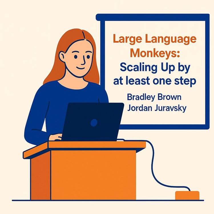
Test-Time Compute Scaling: Smarter LLMs Without Retraining (Video Course)
Your model might already know how to solve your hardest problems,it just hasn't shown you yet. Learn how test-time compute scaling lets small models beat frontier ones. Repeated sampling, verifiers, and the math that makes it predictable.
Related Certification: Certification in Scaling Test-Time Compute for Smarter LLMs
Also includes Access to All:
What You Will Learn
- Explain test-time compute scaling and the three LLM development stages
- Apply repeated sampling and verifier selection to increase pass@k coverage
- Predict sample counts and cost using inference scaling laws
- Design verifiers and use ORMs/PRMs, beam search, and unit tests for selection
- Balance parallel sampling and sequential revision by problem difficulty
- Compose inference pipelines (generation, fusion, critique, ranking) and search them with Archon
Study Guide
Introduction: The Hidden Lever in Your AI Stack
Here's something that might bend your brain a little. The model you're using right now,the one you've been prompting, the one you've been frustrated with, the one you've been told is "limited" by its size,might already know how to solve your hardest problems. It just hasn't shown you yet.
That's the core insight behind test-time compute scaling, and it's one of the most important ideas in AI right now. For years, the assumption was simple: if you want a smarter model, you need a bigger model. More parameters. More pre-training. More billions of dollars spent on GPU clusters humming in some desert data center.
But there's another way. Instead of changing the model, you change how you use it. Instead of asking once and accepting whatever comes back, you ask a hundred times. You generate, you critique, you revise, you fuse. You spend compute at inference time,the moment the model is actually answering,and you extract capability that was already latent in the weights.
This course walks you through the entire paradigm. You'll learn the three stages of LLM development and why the third stage has been underutilized for too long. You'll learn the "Large Language Monkeys" approach to repeated sampling and why it can make a small open-source model beat a frontier proprietary one. You'll learn the scaling laws that make this behavior predictable, the verification problem that makes it hard, and the architecture search frameworks that put it all together.
By the end, you'll understand something most people don't: capability can be purchased with compute at inference time, not just with parameters at training time. That changes the economics of AI for everyone.
Stage One: The Way AI Models Were Built
Every large language model you've ever interacted with went through three distinct phases before it reached your chat window. Understanding these phases is essential, because the entire test-time scaling paradigm is really about rebalancing where we spend our compute.
Pre-training is the monster phase.
This is where the model consumes trillions of tokens of text,books, code, Wikipedia, scientific papers, everything. It runs for months on massive GPU clusters. The compute bill is astronomical. A single pre-training run for a frontier model can cost tens or even hundreds of millions of dollars. This is where the model builds its foundational knowledge, its linguistic ability, its raw reasoning capacity. Nothing about test-time scaling replaces this. It builds on top of it.
Fine-tuning is the refinement phase.
After pre-training, the model gets adapted to specific tasks or behavioral guidelines. This uses orders of magnitude less data,thousands or millions of examples instead of trillions of tokens. It's cheaper, faster, and more targeted. Instruction following, safety alignment, task-specific skills,these all come from fine-tuning. But again, this phase modifies the model's parameters. It changes what the model is.
Inference is the deployment phase.
This is where the model actually answers questions. Historically, inference was treated as a single, lightweight query-response interaction. You send a prompt, the model generates a response, done. Minimal compute per call. A single forward pass. The assumption baked into this design was that inference is a fixed cost,you ask, it answers, you move on.
That assumption is exactly what test-time compute scaling destroys.
The new paradigm says: what if inference isn't a single pass? What if we deliberately spend ten times, a hundred times, or a thousand times more compute at inference time to get a better answer? What if we generate fifty responses and pick the best one? What if we generate a response, critique it, revise it, and repeat? What if we combine multiple models into a pipeline where each one plays a different role?
None of this changes the model's weights. The model stays frozen. But the system's performance changes dramatically. That's the shift. And it matters because it means the intelligence you can deploy isn't locked to the size of the model you can afford to train. It's locked to the cleverness of your inference strategy.
The Large Language Monkeys: Sampling Your Way to Smarter Answers
Let's start with the simplest and most powerful technique in the test-time scaling toolbox: repeated sampling. The name comes from the infinite monkey theorem,give a million monkeys typewriters and eventually they'll produce Shakespeare. Give an LLM enough attempts and eventually it'll produce the right answer.
The procedure is almost embarrassingly simple. Take a problem. Generate multiple responses,ten, a hundred, a thousand. Then use a verifier to select the correct or best response. That's it. That's the whole method.
Why does this work? Because smaller models often "know" the answer to a hard problem without being able to produce it reliably on the first try. The knowledge is latent,buried in the parameters, waiting for the right combination of tokens to surface it. Repeated sampling gives the model multiple chances to find that combination.
Here's a concrete example. Imagine a model with a pass@1 of 0.3 on a given problem,meaning it solves the problem correctly 30% of the time on a single attempt. If you generate 10 independent samples, the probability that at least one is correct is:
1 - (1 - 0.3)¹⁰ = 1 - 0.7¹⁰ ≈ 0.972
You just went from a 30% chance to a 97.2% chance without touching the model. That's the mathematical engine behind this entire approach.
The empirical results are striking. Research has shown that models like Llama 3-8B and Llama 3-70B, which are less capable than GPT-4o on a single attempt, can close the gap significantly,or even overtake it,when allowed to sample repeatedly with a good verifier. The same pattern holds for DeepSeek-V3. On SWE-bench, a benchmark that simulates real software engineering work where an agent edits code and creates patches, DeepSeek-V3 generating 1,000 samples per problem solved more problems than Claude 3.5 or o1-preview on their single-attempt baselines.
Let me give you a second example. Imagine you're working on a coding problem. You ask a model to write a function that checks whether a string of brackets is balanced. On the first try, it might produce a solution that misses an edge case. On the second try, it might handle the edge case but introduce a bug elsewhere. On the fifth try, it nails it. If you have a unit test that verifies correctness, you can automatically identify that fifth response as the winner. Without repeated sampling, you'd never see it.
This works across domains,math, coding, general reasoning, even agentic benchmarks. And critically, in domains with reliable automated verifiers, the entire pipeline runs end-to-end without human intervention. Generate many samples, run the tests, pick the one that passes. That's automation. That's a self-improving system.
Inference Has Scaling Laws Too
Pre-training has well-established scaling laws. Double the compute, double the data, double the parameters, and you can predict how much the loss will drop. It's a reliable, almost boringly predictable relationship. What most people don't realize is that inference-time compute follows its own scaling law,and it's just as predictable.
The relationship between coverage and the number of samples follows an exponential power law. Coverage, in this context, means the fraction of problems solved correctly by at least one of your k samples. The formula looks like this:
coverage(k) = 1 - a . e^(-b.k)
Where a and b are curve-fitting parameters that depend on the model and the task. This isn't a vague hand-wave. It's a mathematical relationship that has been validated across model families,Llama, Gemma, Pythia,across parameter counts from 70 million to 70 billion, and across domains including math, coding, and reasoning.
What does this mean in practice? It means you can plan. If you know your model and your task, you can predict how many samples you'll need to hit a target coverage level. You can estimate the compute cost before you spend it. Inference stops being a fixed cost and becomes a tunable resource,a dial you can turn based on your accuracy requirements and your budget.
Here's an example. Suppose your curve-fitting gives you a = 1.0 and b = 0.05. You want to know how many samples you need to reach 90% coverage. You solve for k:
0.90 = 1 - e^(-0.05.k)
e^(-0.05.k) = 0.10
-0.05.k = ln(0.10)
k ≈ 46
Forty-six samples. That's your answer, before you spend a single GPU cycle. That's the power of a scaling law. And this predictability holds even for surprisingly small models,models with as few as 70 million parameters exhibit the same scaling behavior. The law isn't a privilege of giant models. It's a property of the sampling process itself.
Let me give you another example to make this tangible. Say you're building a system that extracts structured data from legal documents. You test your model on a sample of documents and find that it gets 40% right on a single attempt. You generate 20 samples per document and use a verifier to select the best one. Your coverage jumps to 85%. You generate 100 samples and it jumps to 96%. The scaling law tells you that going from 100 to 200 samples might only buy you another 1.5%,so you can decide whether that's worth the cost. That's the kind of decision this law enables.
The Long Tail of Hard Problems
But here's the deeper question: why does this power law emerge at all? For an individual problem, the relationship between samples and success probability is a simple exponential,pass@k = 1 - (1 - p)^k. That's not a power law. The power law only appears when you aggregate across a whole dataset of problems. And the necessary and sufficient condition for it to appear is the presence of a long tail of hard problems.
Think about a typical dataset. Most problems are relatively easy,the model solves them on the first try. A smaller but significant fraction are harder, requiring a few samples. And a tiny but stubborn tail of problems are extremely difficult, with pass@1 probabilities near zero. These are the problems that only get solved once in a thousand attempts, or ten thousand.
This long tail is what produces the smooth, predictable scaling curve. It's also what makes repeated sampling work at all. If every problem were equally easy, you'd hit 100% coverage after a handful of samples and the curve would flatten instantly. The long tail is what keeps the gains coming as you scale your sample count.
Here's a concrete way to visualize it. Imagine you plot every problem in a dataset on a graph. The x-axis is problem difficulty, measured by pass@1. The y-axis is how many problems sit at that difficulty level. For most datasets, you'd see a curve that starts high on the left,lots of easy problems,and then stretches out to the right, getting thinner and thinner but never quite reaching zero. That thin stretch is the long tail. It's where the hard problems live. And it's those problems, the ones that only get solved once in a blue moon, that determine the shape of your scaling curve.
Empirical analysis of real datasets confirms this condition holds. Most problems are solved at pass@1, but a long tail of increasingly difficult problems requires more samples. This distribution explains why repeated sampling yields diminishing returns,each additional sample solves fewer new problems than the last,yet still produces steady gains as sample counts scale. The tail keeps giving, just more slowly each time.
The Verifier Problem: Generation Is Easy, Verification Is Hard
Here's the uncomfortable truth about repeated sampling: generating a hundred responses is the easy part. Knowing which one is correct is the hard part. The entire approach collapses without a good verifier.
Verification looks very different depending on the domain. Let's walk through the spectrum.
Full verification domains are the gold standard.
In these domains, correctness can be checked objectively. Formal mathematics, for instance, can be verified with proof assistants that mechanically check each logical step. Coding can be verified with unit tests,you write a test, run the code, and see if it passes. There's a particularly elegant example in compiler-level code generation: if you ask a model to generate CUDA code from PyTorch source code, you can verify correctness by running both and comparing their outputs for arbitrary inputs. That's a perfect verifier,objective, automated, and complete. The same principle applies to code porting, like translating Python to C++. Write both, run both, compare.
Language translation is another domain where equivalence checking works. Translate a document from English to French, translate it back, and compare the meaning. Imperfect, but useful as a verification signal.
Let me give you a second example of a full verification domain. On the KernelBench benchmark, models are asked to generate CUDA kernels from PyTorch source code. The verification process is beautifully simple: compile the generated CUDA code, run it on arbitrary inputs, and compare the outputs against the original PyTorch implementation. If they match, the code is correct. This gives researchers a "perfect verifier" by construction. And what do they find? The same linear improvement in coverage with increasing samples. Every additional sample has a chance of being correct, and the verifier catches it every time.
Then there are the challenging verification domains.
General question answering. Open-ended reasoning. Creative writing. There's no unit test for "is this a good essay." No formal proof for "is this the right answer to a complex reasoning question." In these domains, practitioners fall back on proxy methods, and every single one of them is flawed.
Majority voting is the simplest proxy. Generate ten responses, pick the answer that appears most frequently. It works surprisingly well for easy problems, but it has a hard ceiling. Research shows it tends to plateau after roughly ten to fifty samples, especially on easier datasets like GSM8K. And on harder datasets, it performs poorly.
Learned reward models,outcome reward models (ORMs) and process reward models (PRMs),do better, but they still fall short. And this shortfall has a name: the generation-verification gap.
The generation-verification gap is the difference between true coverage,the fraction of problems for which a correct answer exists among your samples,and what your selection method actually captures. It's the distance between what the model could achieve with a perfect verifier and what it achieves with the verifier you actually have. And it's large.
Let me give you a concrete example. On the MATH dataset, which contains hard competition-style problems, researchers generated 10,000 samples per problem. The true coverage,the fraction of problems solved by at least one sample,was far higher than what majority voting could select. Why? Because for the hardest problems, the correct answer appeared only once or twice in those 10,000 samples. Majority voting selects the most frequent answer. A correct answer that appears once is invisible to it.
Here's a second example. On GSM8K, an easier dataset, majority voting handles most problems fine. But even there, the hardest problems in the dataset,the ones with the lowest pass@1,have correct answers that appear rarely. Majority voting misses them. The pattern is consistent: the harder the problem, the wider the gap.
This is why the research community has started saying that generation is not the bottleneck,verification is. We can generate correct answers. We just can't always recognize them. And if you're building real systems, this gap is the difference between a demo that looks impressive and a product that actually works.
Reward Models: Teaching Machines to Judge
Since perfect verifiers don't exist for most domains, we train models to approximate them. These are called reward models, and they come in two flavors.
Outcome reward models (ORMs) score the final answer of a generated response. You generate n responses, feed each one to the ORM, and it outputs a quality score. Then you pick the highest-scoring response. This is called best-of-n selection, and it's the most straightforward way to use an ORM.
Process reward models (PRMs) work differently. Instead of scoring the final answer, they score each individual step of a solution. This enables a much more interesting technique: beam search. At each step of generation, you create several candidate continuations, score them all with the PRM, keep the top-scoring ones, and continue expanding from those. Unpromising branches get pruned early, so your compute focuses on the paths most likely to lead to a correct answer.
Let me walk through a concrete beam search example. Say you have a compute budget of four samples per level. You start by generating four partial solutions to a math problem. The PRM scores each one. You keep the top two. You expand each of those two with new steps, generating four continuations total. The PRM scores those. You keep the top two. You repeat until the solution is complete. At every step, the PRM is guiding you toward the most promising branches of the solution tree.
Here's a second example to show the difference between ORMs and PRMs in practice. Imagine a model solving a multi-step algebra problem. An ORM sees the final answer,say, x = 7,and scores it. If the answer is wrong, the ORM gives you no information about where the solution went wrong. A PRM, on the other hand, scores each step. It might give step one a high score, step two a high score, and step three a low score. That tells you the error happened in step three. You can then revise just that step instead of regenerating the entire solution. That granularity is what makes PRMs so valuable for guiding search.
The trade-off between ORMs and PRMs is worth understanding. ORMs are simpler and cheaper to train, but they only give you a final verdict. PRMs give you granular feedback at every step, which makes them more useful for guiding search. But they're harder to train, and they tend to work best in-domain. A PRM trained on math problems might not generalize perfectly to coding or reasoning tasks.
There's also a hybrid approach that's worth mentioning: generate multiple parallel samples, apply sequential revision to each one, use a PRM to guide the revision process, and select the final answer with an ORM. This combination of parallel exploration and sequential refinement is often the most effective strategy of all.
Sequential Revisions: The Other Dimension of Scaling
Parallel sampling isn't the only way to spend more compute at inference time. There's a second dimension: sequential revision. Instead of generating many independent answers, the model generates one answer and then keeps revising it. It critiques its own output, considers alternative angles, refines its reasoning, and iterates until it's confident in a final answer.
You can induce this behavior with prompting,"review your answer, identify flaws, and improve it",and it's increasingly trained directly into reasoning models. Modern reasoning models don't just produce an answer; they produce a long chain of internal deliberation, checking and re-checking their work.
So now you have two orthogonal ways to scale test-time compute. You can go wide,generate more parallel samples. Or you can go deep,revise sequentially. And the research question becomes: what's the optimal mix?
The answer, it turns out, depends on problem difficulty. This isn't a one-size-fits-all situation.
For easy and medium problems, sequential revision tends to be more efficient.
Why? Because many paths lead to the correct answer. You don't need to explore broadly,you just need to refine what you have. A model can start with a decent approach, critique it, improve it, and converge on the right answer in a relatively small number of tokens. Generating a hundred parallel samples would waste compute when ten sequential revisions would do.
For hard problems, you need parallel exploration.
The correct path isn't obvious. If you start with a single approach and revise it, you might spend forever refining a fundamentally flawed direction. You need many independent attempts to discover even one viable route. Once a viable route is found, sequential revision can refine it,but the discovery phase requires breadth.
Here's a concrete example. Imagine a difficult competition math problem. A single model attempt might go down a dead end,say, trying a substitution technique that doesn't apply. Revising that attempt just produces a more polished dead end. But if you generate fifty parallel attempts, one of them might stumble onto the right approach,say, recognizing the problem as an application of Jensen's inequality. That one attempt can then be revised and refined into a correct solution.
The research on this is remarkably detailed. Studies have binned problems by difficulty and measured the optimal ratio of sequential to parallel compute for each bin. Easy problems favor almost pure sequential refinement. Hard problems require a significant parallel component. And notably, the optimal ratio varies even among hard-problem bins,there's no universal formula yet. This is an open research question.
Let me give you a second example of the difficulty-dependent strategy. Think about customer support tickets. An easy ticket,"how do I reset my password?",can be handled by a single model generating one answer and refining it. A medium ticket,"my account is locked after multiple failed attempts",might benefit from two or three parallel answers that are then critiqued and merged. A hard ticket,"I'm seeing a rare error when integrating your API with my legacy system",benefits from many parallel attempts, each exploring a different hypothesis, before any revision happens. The difficulty of the problem should dictate your sampling strategy.
Test-Time Compute vs. Pre-Training: Where Should You Spend Your Tokens?
Here's a question that keeps engineers up at night: if I have a fixed token budget, should I spend it on inference or on pre-training? Should I take a small model and give it lots of test-time compute, or should I train a bigger model?
The research gives us a nuanced answer. For easy and medium problems, additional test-time compute is more token-efficient than scaling pre-training. You get more bang for your buck by sampling more from a smaller model than by training a larger one. This is huge for organizations that can't afford to pre-train a frontier model. It means you can compete using inference strategies on open-source models.
But for the hardest problems, the calculus flips. Larger models with more pre-training still outperform smaller models even when those smaller models are given large test-time compute budgets. There's a ceiling to what inference scaling can extract from a model. The knowledge simply isn't there for the hardest problems, and no amount of sampling will surface what the model doesn't know.
Let me give you two examples to make this concrete. Example one: a medium-difficulty coding problem. A small open-source model with 1,000 samples and a unit-test verifier will likely solve it. A frontier model on a single attempt might also solve it, but the inference-heavy approach achieves the same result at a fraction of the training cost. Example two: a research-level mathematics problem that requires deep conceptual understanding. A frontier model with massive pre-training has a reasonable chance. A small model, even with 10,000 samples, will keep producing variations of wrong answers,because the underlying reasoning capacity isn't there.
The practical takeaway: test-time scaling is a powerful complement to pre-training, not a replacement. It democratizes capability for most tasks, but the frontier of difficulty still belongs to the biggest models. The smartest strategy uses both levers,pre-training for raw capacity, inference compute for extraction.
The Building Blocks: Seven Operations That Power Inference Architectures
Once you understand repeated sampling and sequential revision, you can start thinking bigger. What if you combined multiple techniques into a pipeline? What if different models played different roles,one generating, another critiquing, another fusing?
This is where test-time scaling becomes a design discipline. Let me introduce the vocabulary. These are the operations that serve as building blocks for inference architectures.
Generation is the atomic unit,standard sampling from a model. You can repeat it n times for parallel scaling. Nothing fancy.
Fusion is where things get interesting. Given k different responses to the same question, you ask an LLM to synthesize a single output, taking all candidates into account. The surprising finding is that fusion often outperforms even oracle selection,that is, picking the single best response with perfect knowledge. Why? Because fusion can combine the strengths of multiple partial answers. One response might have the right approach but a flawed calculation. Another might have the right calculation but a missing step. The fuser can merge them into something better than either.
Critique asks a model to identify the strengths and weaknesses of a given response. This produces structured feedback that can guide improvements. A critic might say, "this proof skips the base case" or "this code fails when the input is empty." That feedback is gold for the next stage.
Ranking asks a model to rank multiple responses by quality. This is a step up from majority voting,instead of counting frequency, you're using the model's judgment. Ranking the top response from a set of candidates beats random selection and provides a solid baseline.
Verification returns a response along with a score and reasoning about why it's correct or incorrect. It's similar to ranking but more explicit about the reasoning behind the judgment.
Unit test generation is a clever trick for coding and math tasks. You ask a model to generate unit tests that encode the problem's requirements. For example, given a problem about balanced round brackets, the model might generate a test like "given a string with an odd number of brackets, output 'no'" or "each closing bracket must match the most recently opened unmatched bracket." These tests encode the problem's constraints in executable form.
Unit test evaluation then asks a model to judge whether a candidate solution passes a generated unit test. Here's the wild part: this works even without executing any code. The model can reason about whether the solution would pass the test. This is especially useful when execution is expensive or impractical.
Let me give you a second example of fusion in action. Say you ask five different models to solve a logic puzzle. Each produces a partially correct answer. Model A gets the first half right, Model B gets the second half right, Model C has the right conclusion but shaky reasoning, Model D is wrong but has an interesting insight, Model E is completely off. A fusion model reads all five and synthesizes a final answer. It can identify the correct elements from A and B, use C's conclusion as a sanity check, and discard the noise from D and E. The fused answer is more robust than any individual response.
And here's a practical tip about fusion: it works even better when you filter before you fuse. Instead of fusing all k responses, rank them first and fuse only the top-k. The ranker removes the noise, and the fuser can focus on combining the strongest candidates. This two-step process,rank, then fuse,consistently outperforms fusing everything.
Archon: Treating Inference as an Architecture Search Problem
Now we get to the most advanced concept in this course. If inference-time operations are building blocks, then the question becomes: how do you combine them? What's the optimal pipeline? And can you search for it automatically?
That's exactly what the Archon framework does. Archon is an architecture search framework for inference-time scaling. It treats the inference pipeline as a design problem,analogous to how neural architecture search treats model design as a problem.
Frequently Asked Questions
Introduction
Test-time compute scaling is one of the most practical levers available for improving AI system performance without touching model weights. This FAQ addresses the questions that surface when you actually try to implement these techniques,from understanding why repeated sampling works to deciding when architecture search makes sense for your budget. The answers progress from foundational concepts through advanced implementation details, so you can find what you need whether you're evaluating the approach for the first time or already building inference pipelines.
What are the three primary stages in the lifecycle of a large language model?
Large language models move through three distinct development phases. Pre-training is the most compute-intensive stage, consuming months of GPU time across massive clusters while the model learns from trillions of tokens. Fine-tuning uses orders of magnitude less data, adapting the pre-trained model for specific behaviors like instruction following or domain expertise. Inference is where the model generates responses to queries,historically a single, cheap forward pass.
Test-time compute scaling changes the economics of the third stage. Instead of one query in and one answer out, you deliberately spend more compute during inference,generating multiple candidates, revising responses, or running verification checks. The model weights stay frozen. All the improvement comes from how you use the model at inference time, which makes this approach accessible to teams that don't have the resources to pre-train frontier-scale models.
What is test-time compute scaling?
Test-time compute scaling refers to any technique that improves model performance by allocating additional computational resources during inference rather than through additional training or fine-tuning. The core insight is that a model's capabilities can be more fully elicited by letting it explore multiple answers, revise its own responses, or use external verifiers.
Three broad categories exist: parallel sampling generates multiple independent responses and selects the best one; sequential revision lets the model iteratively refine its own answer through self-critique or planning; learned selection uses reward models or rankers to choose among candidates. These methods combine well, and they're especially valuable for smaller open-source models that lag behind frontier proprietary models on a single attempt but become competitive with enough inference compute.
How does repeated sampling improve model performance?
Repeated sampling,also called best-of-n sampling,works by generating multiple responses to the same input, then using a verifier to select the correct one. Given a problem, the model produces 10, 100, or 1,000 candidate answers. A verifier evaluates each one, and a correct response is returned as the output.
The results are striking. Smaller models like Llama 3-8B or 70B, which underperform GPT-4o on a single attempt, can match or exceed it on difficult math and coding benchmarks simply by generating many candidates and selecting the right one with a verifier. The model already "knew" the answer,it just didn't produce it on the first try. This works across agentic benchmarks too. On SWE-bench, which simulates a software engineer editing code and creating patches, DeepSeek-V3 with 1,000 samples per problem solved more engineering tasks than Claude 3.5 or o1-preview when unit tests selected the correct patches.
What is "coverage" in the context of repeated sampling?
Coverage measures how many problems in a benchmark are solved by at least one of the generated samples. If you generate k samples per problem, coverage is the fraction of problems for which at least one of those k samples is correct. This is closely tied to the pass@k metric,the probability that at least one of k generated samples solves the problem.
Coverage increases as k increases, but not linearly. The relationship follows a predictable pattern that you can model mathematically. Understanding this curve matters because it tells you how many samples you need to generate to hit a target performance level, which directly determines your compute budget. If you know your model's coverage curve, you can predict whether generating 500 samples gets you to 80% coverage or if you need 2,000.
What scaling law governs coverage as a function of the number of samples?
Researchers have found that coverage follows an exponential power law: Coverage ≈ a × kᵇ, where a and b are curve-fitting coefficients derived from the model's scaling behavior. This law holds across model families (Llama 3, Gemma, Pythia) and sizes from 70 million to 70 billion parameters, across multiple domains.
The practical value is predictive. Given a model and benchmark, you can estimate how many samples you need to achieve a target coverage level and therefore how much compute to budget. The predictions closely match actual observed coverage. Even very small models exhibit this predictable scaling, suggesting that repeated sampling is a general strategy for eliciting capability across model scales,not just a trick that works for large models.
Why does repeated sampling produce a power law rather than a simple exponential curve?
For a single problem where the probability of a correct response is p, the probability that at least one of k samples is correct is 1 - (1 - p)ᵏ,a simple exponential. But across a suite of problems, what emerges is a power law. The reason is the long tail of hard problems in the dataset.
For a power law to emerge, the pass@1 probabilities across problems must follow a long-tail distribution: many easy problems with high pass@1, and a steadily decreasing tail of harder problems with very low pass@1. This is exactly what researchers observe empirically. The practical implication is that repeated sampling works best when a model has at least some probability of solving every problem. The hard-tail problems get solved only rarely, but given enough samples, they eventually get captured.
What is pass@k and how does it differ from coverage?
Pass@k is the probability that at least one of k generated samples correctly solves a given problem. For an individual problem with pass@1 = p, pass@k = 1 - (1 - p)ᵏ. Coverage extends this concept across a whole benchmark,it's the fraction of problems where at least one of k samples is correct.
The distinction matters when you're setting evaluation targets. Pass@k tells you about a single problem's likelihood of being solved. Coverage tells you about system-level performance across many problems. If you're building a system that needs to handle a diverse workload, coverage is the metric that matters for business decisions. If you're debugging why a specific problem isn't being solved, pass@k is more useful for isolating the issue.
Where does the "Large Language Monkeys" name come from?
The name references the infinite monkey theorem,the idea that a monkey hitting keys at random on a typewriter will eventually produce a complete work of literature given infinite time. The analogy applies to LLMs: given enough random attempts, even an unlikely correct answer will eventually appear.
In practice, this means generating many independent responses to the same problem and using a verifier to identify the correct one. The name captures the essence of the approach,brute-force exploration of the output space,while acknowledging that the "randomness" is actually guided by the model's learned distribution. The model isn't generating random text; it's sampling from a distribution that contains correct answers, just not always on the first attempt. The method is about surfacing those latent correct answers through volume.
What role do verifiers play in test-time compute scaling?
Verifiers are the backbone of repeated sampling. If you generate many candidate responses, you need a way to determine which ones are correct. The quality of the verifier directly determines the quality of the final output.
Some domains make verification straightforward: mathematics can use formal proof assistants; coding can use unit tests; compiler code generation (like converting PyTorch to CUDA) can compare outputs for all inputs, providing a "perfect" automatic verifier. Other domains lack reliable verifiers, which creates the generation-verification gap. The availability of a good verifier is often the deciding factor in whether repeated sampling will work in a given domain. If you can't verify answers, generating more samples doesn't help,you can't tell which one is right.
What is the generation-verification gap?
The generation-verification gap is the difference between what you'd achieve with a perfect verifier (true coverage) and what you actually achieve with practical selection methods like majority voting or reward model rankers. Even well-trained reward models leave a large gap, and it widens on harder problems.
On the MATH benchmark, majority voting plateaus after just 10-50 samples while true coverage keeps climbing. Reward-model-based methods do better but still leave significant performance unrealized. This gap represents lost potential,correct answers exist in your sample pool, but your selection mechanism can't identify them. Closing this gap is one of the most active research areas in test-time compute scaling. For practitioners, it means you should measure your actual achieved accuracy, not just theoretical coverage, when evaluating whether repeated sampling is working for your use case.
Why does majority voting fail on hard problems?
Majority voting selects the answer that appears most frequently among generated samples. It works when correct answers are common. It fails on hard problems because correct answers are rare.
For the hardest problems in a benchmark, the correct solution might appear only once or twice out of 1,000 or even 10,000 samples. Since minority answers are by definition not the majority, majority voting will never select them. On easier problems like those in GSM8K, correct answers appear frequently enough that majority voting works reasonably well. But even there, the hardest fraction of problems has correct answers that are too rare for frequency-based selection. This is why verifiers or reward models are necessary,they can identify a single correct rare answer, whereas frequency-based methods cannot.
What are the two main modes of allocating test-time compute?
The two primary modes are parallel sampling and sequential revision. Parallel sampling generates many independent responses to the same input, exploring the model's output distribution broadly. Sequential revision starts with an initial solution and iteratively refines it,self-correcting, examining the problem from different angles, and continuing until the model is confident enough to produce a final answer.
Modern reasoning models are trained to exhibit sequential revision behavior internally, but it can also be prompted explicitly. A third dimension is answer selection: how you choose among generated responses using outcome reward models, process reward models, or other ranking methods. Most effective strategies blend both modes,generating a few parallel samples, then applying sequential revision to each one, guided by reward models.
What is the difference between outcome reward models and process reward models?
Outcome reward models (ORMs) score the final response as a whole. They take a question and a complete answer and produce a score indicating correctness likelihood. They're used for best-of-n selection: generate n samples, score each with the ORM, return the highest-scoring one.
Process reward models (PRMs) score each individual step of a solution. A math solution with five steps gets five separate quality scores. PRMs are typically fine-tuned language models trained on human annotations of step-level correctness. They're more useful than ORMs for search-based test-time scaling because they guide generation at intermediate stages, not just at the end. They also generalize better to new tasks since they're language-model based, though they perform best on domains they were trained on.
How can process reward models guide test-time scaling?
A common technique is beam search guided by a PRM. Given a question, you generate an initial set of candidate steps (say, 4 samples), score each using the PRM, keep only the top 2, then continue generating steps from those survivors. Repeat until a final answer is produced.
At each level of the search tree, the PRM prunes unpromising branches, focusing compute on the most promising solutions. This is analogous to beam search in traditional sequence generation. Many off-the-shelf PRMs exist, and you can also train your own on your own data. The quality of the PRM matters enormously,a good one substantially improves the efficiency of test-time compute, while a poor one wastes compute on bad branches. The step-level feedback is what makes PRMs powerful: they catch errors early before they compound into a completely wrong final answer.
How do you train a process reward model?
PRMs are typically fine-tuned from base language models using step-level human annotations. You collect solutions to problems, break them into steps, and have annotators label each step as "good" or "bad." This produces a training dataset where the model learns to score individual reasoning steps rather than whole answers.
Synthetic data generation is increasingly used to reduce annotation costs. You can generate many candidate solutions, use automated verifiers (like unit tests for code or formal proof checkers for math) to identify correct and incorrect solutions, then align individual steps with the final outcome. The key is that PRMs need to learn what makes a step good in isolation, not just in context of the final answer. A step might be locally correct but lead to a dead end, or locally questionable but part of a valid solution path. Training data should capture both cases.
How does problem difficulty affect the optimal test-time scaling strategy?
Research shows the optimal balance between sequential revision and parallel sampling depends on problem difficulty. For easy and medium problems, sequential test-time compute is very effective and more token-efficient than generating many parallel samples. Most paths lead to the correct answer, so focusing compute on refining one solution works.
For hard problems, greater parallel exploration is necessary because many candidate solutions are dead ends. You need to explore a wide variety of approaches to find one that works. Comparing test-time compute to pre-training compute, additional test-time compute is more favorable than scaling model parameters for easy and medium questions. But for the hardest problems, larger models with more pre-training still outperform smaller models even with very large test-time budgets. Test-time scaling makes modest models useful for most tasks, but frontier models remain necessary for the hardest reasoning challenges.
Can test-time compute scaling replace pre-training?
Not entirely. For many problems,especially easy and medium ones,test-time scaling is so effective that smaller open-source models can match or exceed larger proprietary models. This makes pre-training a less critical investment for those tasks, which matters because only a few organizations can afford to pre-train frontier-scale models.
However, for the hardest problems, evidence indicates that additional pre-training (producing larger, more knowledgeable models) still outperforms any reasonable amount of test-time compute applied to a smaller model. Test-time scaling is a powerful complement, not a replacement. The practical strategy is to use test-time scaling to maximize the value of models you already have, while recognizing that the hardest problems in your domain may still require investment in better base models.
How does test-time compute scaling differ from chain-of-thought prompting?
Chain-of-thought (CoT) prompting asks the model to show its reasoning steps before giving a final answer. It's a single-pass technique,the model generates a reasoning trace and conclusion in one forward pass. Test-time compute scaling goes further by allocating additional compute across multiple inference passes.
CoT is one technique within the test-time scaling toolbox. It's the foundation for sequential revision,you can't iteratively refine an answer without first generating a reasoning trace. But test-time scaling adds the dimension of multiple attempts: generating many CoT traces in parallel, scoring them with verifiers or reward models, fusing the best ones, or revising them sequentially. CoT is deterministic per sample; test-time scaling introduces selection and iteration. Think of CoT as the reasoning primitive and test-time scaling as the system that orchestrates multiple reasoning attempts to maximize the chance of a correct answer.
What is self-consistency and how does it relate to repeated sampling?
Self-consistency generates multiple reasoning paths for the same problem, then selects the most consistent answer across all paths. It was one of the earliest repeated-sampling methods, predating more sophisticated verifier-based approaches. The assumption is that correct answers tend to cluster,multiple independent reasoning paths converge on the same conclusion.
Repeated sampling with verifiers is a generalization of this idea. Instead of relying on answer frequency, you use a learned verifier or external check (like unit tests) to identify the correct answer. Self-consistency is essentially majority voting over reasoning paths, which means it inherits the same limitations on hard problems,rare correct answers get outvoted. But it's a useful baseline and works well on easier problems where correct answers are more common. Modern approaches use reward models or process reward models instead of frequency-based selection to capture rare correct answers.
Certification
About the Certification
Become certified in test-time compute scaling and prove you can make smaller LLMs beat frontier ones. You'll know when to scale sampling, build verifiers, and predict compute gains,then apply it to real inference pipelines.
Official Certification
Upon successful completion of the "Certification in Scaling Test-Time Compute for Smarter LLMs", you will receive a verifiable digital certificate. This certificate demonstrates your expertise in the subject matter covered in this course.
Benefits of Certification
- Enhance your professional credibility and stand out in the job market.
- Validate your skills and knowledge in cutting-edge AI technologies.
- Unlock new career opportunities in the rapidly growing AI field.
- Share your achievement on your resume, LinkedIn, and other professional platforms.
How to complete your certification successfully?
To earn your certification, you’ll need to complete all video lessons, study the guide carefully, and review the FAQ. After that, you’ll be prepared to pass the certification requirements.
Other AI Video Courses
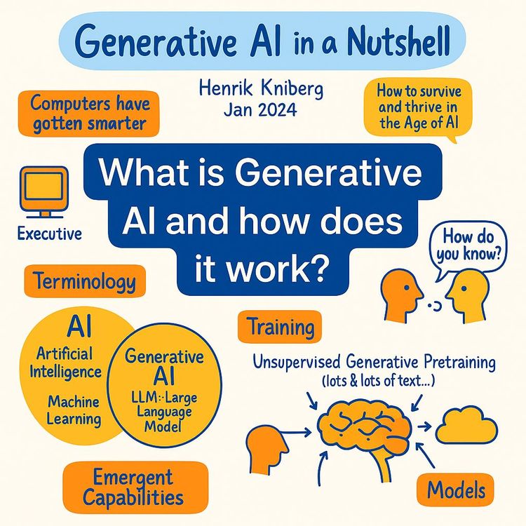
Video Course: What is Generative AI and how does it work?

Video Course: How to Use ChatGPT from Beginner to Professional

Video Course: How to Use Google Gemini for Google Workspace to Boost Productivity

Video Course: How to Use Claude 3.7 AI - Tips for Beginners!

Video Course: ChatGPT for Data Analytics: Full Course - from Beginners to Professional

Video Course: Generating Images and photos With ChatGPT?

Video Course: Generating Images & Photo's with MidJourney

Video Course: Generating Design's with Microsoft Designer and AI

Video Course: Generating Design's with Canva.com and AI
Join 20,000+ Professionals, Using AI to transform their Careers
Join professionals who didn’t just adapt, they thrived. You can too, with AI training designed for your job.