
Video Course: Linear Algebra Course – Mathematics for Machine Learning and Generative AI
Delve into the essential mathematics of Machine Learning and Generative AI with our Linear Algebra course. From foundational ideas to advanced applications, gain a robust understanding of how these concepts drive modern AI technologies.
Related Certification: Certified Linear Algebra for Machine Learning & Generative AI

Also includes Access to All:
What You Will Learn
- Visualize and manipulate vectors in Rn
- Compute norms, dot products, distances, and angles
- Perform matrix operations and solve Ax = b
- Understand eigenvalues, eigenvectors, and PCA basics
- Represent real-world data as vectors and exploit sparsity
Study Guide
Introduction
Welcome to the comprehensive video course on Linear Algebra, designed specifically for those interested in the mathematics underpinning Machine Learning and Generative AI. This course is crafted to take you from foundational concepts to advanced applications, ensuring a deep understanding of how linear algebra plays a crucial role in modern AI technologies. By the end of this course, you'll be equipped with the knowledge to apply linear algebra concepts effectively in various AI contexts.
Foundational Concepts
Coordinate Systems
Understanding coordinate systems is essential for visualizing vectors and performing operations in multidimensional spaces. In a two-dimensional coordinate system, also known as a Cartesian plane, we have two perpendicular axes: the x-axis (horizontal) and the y-axis (vertical). The intersection of these axes is the origin, denoted as (0, 0). This system allows us to uniquely identify any point in 2D space using an ordered pair of numbers (x, y), which represent its position relative to the origin.
In three-dimensional space, we introduce a third axis, the z-axis, which is perpendicular to both the x and y axes, allowing us to describe points in 3D space as (x, y, z). This concept extends to n-dimensional space (Rⁿ), where each point is described by an n-tuple of real numbers.
Example 1: Consider a point P in 2D space with coordinates (3, 4). This means P is located 3 units along the x-axis and 4 units along the y-axis from the origin.
Example 2: In 3D space, a point Q with coordinates (2, -1, 5) is 2 units along the x-axis, -1 unit along the y-axis, and 5 units along the z-axis.
Visualizing vectors in these spaces is crucial for understanding their geometric properties and performing vector operations.
Basic Trigonometry and Geometry
Trigonometry is the study of relationships between the angles and sides of triangles, and it is fundamental in linear algebra for understanding vector directions and transformations.
The basic trigonometric functions are sine (sin), cosine (cos), and tangent (tan). For an angle θ in a right triangle:
- Sine (sin θ) = Opposite side / Hypotenuse
- Cosine (cos θ) = Adjacent side / Hypotenuse
- Tangent (tan θ) = Opposite side / Adjacent side
The Pythagorean theorem states that in a right-angled triangle, the square of the hypotenuse (c) is equal to the sum of the squares of the other two sides (a and b): a² + b² = c².
These concepts are crucial for calculating vector magnitudes, directions, and performing transformations.
Example 1: To find the length of a vector (3, 4) in R², use the Pythagorean theorem: √(3² + 4²) = √(9 + 16) = 5.
Example 2: The angle between two vectors can be found using cos θ = (A · B) / (||A|| ||B||), where A · B is the dot product of vectors A and B.
Real Numbers and Vector Spaces
The set of all real numbers (R) includes integers, negative numbers, and floating-point numbers. In a one-dimensional space, we deal with single real numbers. The concept extends to R², R³, ..., Rⁿ, representing n-dimensional Euclidean spaces. For instance, R² is a 2D plane where each point can be described by an (x, y) coordinate pair.
Example 1: In R², a vector (1, 2) represents a point 1 unit along the x-axis and 2 units along the y-axis.
Example 2: In R³, a vector (3, 0, -1) represents a point 3 units along the x-axis, 0 units along the y-axis, and -1 unit along the z-axis.
Understanding these spaces is crucial for modeling and solving problems in higher dimensions, which is common in machine learning and AI.
Vectors
Definition and Representation
A vector is an entity with both magnitude (length) and direction, distinguishing it from a scalar, which only has magnitude. Vectors can be visualized as arrows in a coordinate system, where the starting point is not as important as the magnitude and direction.
In 2D space, vectors are represented using parentheses or square brackets, e.g., (4, 0) or [3, 4]. In n-dimensional space (Rⁿ), a vector is represented as a column of n elements:
[ A₁ ]
[ A₂ ]
[ ... ]
[ Aₙ ]
Example 1: A vector (5, -3) in R² represents a point 5 units along the x-axis and -3 units along the y-axis.
Example 2: In R³, a vector (2, 1, 4) can be visualized as an arrow from the origin to the point (2, 1, 4).
Indexing
In an n-dimensional vector, the standard mathematical notation for indices goes from i = 1 to n. Aᵢ refers to the i-th element of vector A. When dealing with collections of vectors, notation like Aᵢ with an arrow might represent the i-th vector in the collection, where each Aᵢ is itself a vector.
Example 1: For a vector A = [3, 5, 7], A₂ = 5 is the second element.
Example 2: In a collection of vectors [A₁, A₂, A₃], A₂ could be a vector like [4, 0, -2].
Special Vectors
Several types of vectors have special properties:
- Zero Vector: A vector where all its elements are zero. For example, in R³, the zero vector is [0, 0, 0].
- Unit Vectors: Vectors with a single element equal to one and all other elements zero. The i-th unit vector in n dimensions is denoted as Eᵢ.
- Sparse Vectors: Vectors characterized by having many of their entries as zero. The sparsity pattern indicates the positions of non-zero entries.
Example 1: The zero vector in R² is [0, 0].
Example 2: The unit vector E₁ in R³ is [1, 0, 0].
Vector Operations
Addition and Subtraction
Two vectors of the same size are added (or subtracted) by adding (or subtracting) their corresponding elements. The resulting vector has the same size. Vector addition is commutative (A + B = B + A) and associative ((A + B) + C = A + (B + C)). There exists an additive identity (zero vector) such that A + 0 = A, and every vector has an additive inverse (-A) such that A + (-A) = 0.
Example 1: Adding vectors A = (2, 3) and B = (1, 4) results in A + B = (3, 7).
Example 2: Subtracting vector B = (1, 4) from A = (2, 3) results in A - B = (1, -1).
Scalar Multiplication
Multiplying a vector by a scalar involves multiplying each component of the vector by that scalar, effectively scaling the vector's magnitude. The direction remains the same if the scalar is positive and reverses if the scalar is negative. Multiplying a vector by zero results in the zero vector.
Example 1: Multiplying vector A = (2, 3) by 2 results in 2A = (4, 6).
Example 2: Multiplying vector B = (1, 4) by -1 results in -B = (-1, -4).
Application: Audio Scaling
Scalar vector multiplication can be used in audio processing to change the volume of an audio signal (represented as a vector) without altering its content. Multiplying by a scalar greater than 1 increases the volume, while multiplying by a scalar between 0 and 1 decreases it. A negative scalar would also invert the phase of the audio.
Example 1: If an audio signal is represented by a vector A = (0.5, 0.7, 0.6), multiplying by 2 increases the volume to (1.0, 1.4, 1.2).
Example 2: Multiplying the same audio signal by 0.5 decreases the volume to (0.25, 0.35, 0.3).
Span and Linear Combination
Linear Combination
A linear combination of vectors is formed by taking a set of vectors, multiplying each by a scalar, and then adding the resulting scaled vectors together. This concept is fundamental in defining vector spaces and subspaces.
Example 1: For vectors A = (1, 2) and B = (3, 4), a linear combination could be 2A + 3B = 2(1, 2) + 3(3, 4) = (2, 4) + (9, 12) = (11, 16).
Example 2: For vectors C = (0, 1) and D = (1, 0), a linear combination could be 5C - D = 5(0, 1) - (1, 0) = (0, 5) - (1, 0) = (-1, 5).
Span
The span of a set of vectors is the set of all possible linear combinations that can be formed from those vectors. It represents the subspace that can be reached by scaling and adding the given vectors.
Example 1: The span of vectors (1, 0) and (0, 1) in R² is the entire 2D plane, as any vector in R² can be expressed as a linear combination of these two.
Example 2: The span of vectors (1, 1) and (2, 2) is a line through the origin, as any linear combination of these vectors lies on the line y = x.
Linear Dependence and Independence
A set of vectors is linearly dependent if at least one vector in the set can be expressed as a linear combination of the others. If no vector can be expressed as a linear combination of the others (the only linear combination that equals the zero vector is the trivial one where all scalars are zero), then the set is linearly independent.
Example 1: Vectors (1, 2), (2, 4), and (3, 6) are linearly dependent because (2, 4) = 2(1, 2) and (3, 6) = 3(1, 2).
Example 2: Vectors (1, 0) and (0, 1) are linearly independent because no vector can be expressed as a scalar multiple of the other.
Length of a Vector (Norm) and Dot Product
Norm (Magnitude or Length)
The norm of a vector (often the L2 norm or Euclidean norm) measures its size or length. For a vector v = [v₁, v₂, ..., vₙ]ᵀ, the L2 norm is calculated as:
||v||₂ = √(v₁² + v₂² + ... + vₙ²)
Example 1: For vector v = (3, 4), the norm is ||v|| = √(3² + 4²) = √(9 + 16) = 5.
Example 2: For vector w = (1, 2, 2), the norm is ||w|| = √(1² + 2² + 2²) = √(1 + 4 + 4) = 3.
Euclidean Distance
The Euclidean distance between two points A and B in n-dimensional space is the norm of the vector connecting A to B. If A = [A₁, A₂, ..., Aₙ]ᵀ and B = [B₁, B₂, ..., Bₙ]ᵀ, the Euclidean distance is calculated as:
d(A, B) = √((A₁ - B₁)² + (A₂ - B₂)² + ... + (Aₙ - Bₙ)²)
Example 1: The distance between points (1, 2) and (4, 6) is √((4 - 1)² + (6 - 2)²) = √(3² + 4²) = 5.
Example 2: The distance between points (1, 0, 3) and (4, 5, 6) is √((4 - 1)² + (5 - 0)² + (6 - 3)²) = √(3² + 5² + 3²) = √(9 + 25 + 9) = √43.
Dot Product
The dot product of two n-dimensional vectors A = [A₁, A₂, ..., Aₙ]ᵀ and B = [B₁, B₂, ..., Bₙ]ᵀ is defined as:
AᵀB = A₁B₁ + A₂B₂ + ... + AₙBₙ
The dot product of a vector with itself (VᵀV) is equal to the square of its L2 norm (||V||₂²).
Example 1: The dot product of vectors A = (1, 2) and B = (3, 4) is 1*3 + 2*4 = 3 + 8 = 11.
Example 2: The dot product of vectors C = (1, 0, -1) and D = (2, -1, 3) is 1*2 + 0*(-1) + (-1)*3 = 2 + 0 - 3 = -1.
Geometric Interpretation of Dot Product
The dot product is related to the angle (θ) between two vectors: AᵀB = ||A|| ||B|| cos(θ). This shows how the dot product can be used to measure the similarity or relationship between two vectors. If the dot product is zero, the vectors are orthogonal (perpendicular, θ = 90°).
Example 1: Vectors (1, 0) and (0, 1) are orthogonal because their dot product is 0.
Example 2: Vectors (1, 1) and (2, 2) are not orthogonal because their dot product is 1*2 + 1*2 = 4, which is positive.
Linear Systems and Matrices
Representation of Linear Systems
A system of m linear equations with n unknowns can be represented using matrices. The system:
a₁₁x₁ + a₁₂x₂ + ... + a₁nxₙ = b₁
a₂₁x₁ + a₂₂x₂ + ... + a₂nxₙ = b₂
...
aₘ₁x₁ + aₘ₂x₂ + ... + aₘnxₙ = bₘ
can be written in matrix form as Ax = b, where A is the m x n coefficient matrix, x is the n x 1 column vector of unknowns, and b is the m x 1 column vector of constants.
Example 1: The system of equations x + 2y = 5 and 3x + 4y = 6 can be represented as:
A = [ [1, 2], [3, 4] ], x = [x, y]ᵀ, b = [5, 6]ᵀ
Example 2: The system of equations x - y + z = 1, 2x + y + 3z = 4, and -x + 4y + z = 2 can be represented as:
A = [ [1, -1, 1], [2, 1, 3], [-1, 4, 1] ], x = [x, y, z]ᵀ, b = [1, 4, 2]ᵀ
Coefficient Matrix
The matrix A contains the coefficients of the unknowns in the linear equations. The element aᵢⱼ refers to the coefficient in the i-th row (equation) and j-th column (corresponding to the j-th unknown).
Example 1: In the matrix A = [ [1, 2], [3, 4] ], a₁₂ = 2 is the coefficient of y in the first equation.
Example 2: In the matrix A = [ [1, -1, 1], [2, 1, 3], [-1, 4, 1] ], a₃₂ = 4 is the coefficient of y in the third equation.
Homogeneous and Non-Homogeneous Systems
A linear system is homogeneous if all the constant terms (bᵢ) are zero (Ax = 0). Otherwise, it is non-homogeneous (Ax = b where b ≠ 0).
Example 1: The system of equations x + 2y = 0 and 3x + 4y = 0 is homogeneous.
Example 2: The system of equations x + 2y = 5 and 3x + 4y = 6 is non-homogeneous.
Conclusion
Congratulations on completing this comprehensive course on linear algebra tailored for machine learning and generative AI. By mastering these concepts, you now have a solid foundation to understand and implement the mathematical principles that drive AI technologies. Remember, the thoughtful application of these skills is what transforms theoretical knowledge into practical innovations. Continue exploring and applying these concepts to unlock new possibilities in the world of AI.
Podcast
There'll soon be a podcast available for this course.
Frequently Asked Questions
Welcome to the FAQ section for the 'Video Course: Linear Algebra Course – Mathematics for Machine Learning and Generative AI.' This resource is designed to address common questions, clarify concepts, and provide practical insights into how linear algebra is applied in machine learning and generative AI. Whether you're a beginner or an experienced professional, you'll find valuable information to enhance your understanding and application of these mathematical principles.
What are the fundamental components of a two-dimensional coordinate system, and why are they essential for visualising vectors?
A two-dimensional coordinate system, also known as a Cartesian plane, is fundamentally composed of two perpendicular lines called axes: the horizontal x-axis and the vertical y-axis. Their point of intersection is called the origin, often denoted as (0, 0). This system allows us to uniquely identify any point in a two-dimensional space using an ordered pair of numbers (x, y), representing its position relative to the origin along the x and y axes, respectively.
This coordinate system is essential for visualising vectors because a vector in two dimensions can be represented as an arrow originating from one point (often the origin) and terminating at another point (x, y). The coordinates of the endpoint define the vector's components, indicating its magnitude (length) and direction in the 2D space. Without this system, it would be impossible to precisely depict and understand the geometric properties of vectors.
What are the basic trigonometric functions (sine, cosine, tangent) and the Pythagorean theorem, and why is understanding them important in the context of linear algebra and vectors?
The basic trigonometric functions (sine, cosine, tangent) relate the angles of a right-angled triangle to the ratios of its sides. For an angle θ in a right triangle:
Sine (sin θ) is the ratio of the length of the side opposite the angle to the length of the hypotenuse.
Cosine (cos θ) is the ratio of the length of the side adjacent to the angle to the length of the hypotenuse.
Tangent (tan θ) is the ratio of the length of the side opposite the angle to the length of the side adjacent to the angle.
The Pythagorean theorem states that in a right-angled triangle, the square of the length of the hypotenuse (the side opposite the right angle) is equal to the sum of the squares of the lengths of the other two sides (a and b): a² + b² = c².
Understanding these concepts is crucial in linear algebra, particularly when dealing with vectors, for several reasons:
Vector Magnitude: The Pythagorean theorem is used to calculate the magnitude (length) of a vector based on its components in a coordinate system.
Vector Direction: Trigonometric functions are essential for describing the direction of a vector in terms of angles relative to the coordinate axes.
Dot Product: The geometric interpretation of the dot product involves the cosine of the angle between two vectors, linking trigonometry to vector operations.
Transformations: Rotations of vectors in space are often described using trigonometric functions within transformation matrices.
Explain the concept of "R" and how it extends to "R2", "R3", and "Rn". What does each of these spaces represent?
In the context of vector spaces, "R" represents the set of all real numbers. This can be visualised as a one-dimensional space, a number line where every point corresponds to a real number.
R2: "R2" represents the two-dimensional Euclidean space. It consists of all possible ordered pairs of real numbers (x, y). Each pair can be visualised as a point in a two-dimensional Cartesian plane, defined by the x-axis and y-axis. Vectors in R2 can be thought of as arrows in this plane, with two components corresponding to their displacement along the x and y directions.
R3: "R3" represents the three-dimensional Euclidean space. It includes all possible ordered triples of real numbers (x, y, z). Each triple corresponds to a point in a three-dimensional Cartesian space, with x, y, and z axes. Vectors in R3 are arrows in this 3D space, having three components representing their displacement along the x, y, and z axes.
Rn: "Rn" generalises this concept to n-dimensional Euclidean space. It comprises all possible ordered n-tuples of real numbers (x1, x2, ..., xn). While it becomes harder to visualise for n > 3, Rn provides a powerful mathematical framework for dealing with data that has n features or dimensions. Vectors in Rn have n components.
What is a vector, how is it represented in a coordinate system, and what distinguishes it from a scalar?
A vector is a quantity that has both magnitude (length) and direction. It can represent physical quantities like displacement, velocity, and force.
In a coordinate system (e.g., R2 or R3), a vector is typically represented by an arrow that originates from one point (often the origin) and ends at another point. The coordinates of the endpoint relative to the origin define the components of the vector. For example, in R2, a vector might be represented as $\begin{pmatrix} x \ y \end{pmatrix}$ or $(x, y)$, where x and y are the horizontal and vertical components, respectively. The arrow's length corresponds to the vector's magnitude, and the orientation of the arrow indicates its direction.
A scalar, on the other hand, is a single numeric value that represents only magnitude or quantity, without any direction. Examples of scalars include temperature, height, or speed (without direction). In mathematical notation, vectors are often denoted by a letter with an arrow above it (e.g., $\vec{v}$) or in boldface (e.g., $\mathbf{v}$), while scalars are usually represented by regular lowercase letters (e.g., s).
Define the Euclidean norm (or L2 norm) of a vector. How is it calculated, and what does it represent geometrically?
The Euclidean norm (or L2 norm) of a vector is a measure of its length or magnitude in Euclidean space. For a vector $v = \begin{pmatrix} v_1 \ v_2 \ \vdots \ v_n \end{pmatrix}$ in Rn, the Euclidean norm, denoted as $||v||_2$ or simply $||v||$, is calculated as the square root of the sum of the squares of its components:
$||v||_2 = \sqrt{v_1^2 + v_2^2 + \dots + v_n^2}$
Geometrically, in two dimensions (R2), the Euclidean norm of a vector represents the straight-line distance from the origin (0, 0) to the point $(v_1, v_2)$, according to the Pythagorean theorem. In three dimensions (R3), it represents the straight-line distance from the origin to the point $(v_1, v_2, v_3)$. In higher dimensions (Rn), it generalises this concept of distance from the origin to a point in the n-dimensional space.
Explain the concept of Euclidean distance between two points (vectors) in Rn. How is it related to the norm of a vector?
The Euclidean distance between two points (or vectors) A and B in Rn is the length of the straight line segment that connects them. If $A = (a_1, a_2, \dots, a_n)$ and $B = (b_1, b_2, \dots, b_n)$, then the Euclidean distance $d(A, B)$ is calculated as:
$d(A, B) = \sqrt{(a_1 - b_1)^2 + (a_2 - b_2)^2 + \dots + (a_n - b_n)^2}$
The Euclidean distance between two points A and B is fundamentally related to the norm of a vector. Specifically, the distance $d(A, B)$ is equal to the Euclidean norm of the vector that connects A to B. This connecting vector is obtained by subtracting the components of A from the corresponding components of B (or vice versa, since the terms are squared):
Vector connecting A to B = $B - A = \begin{pmatrix} b_1 - a_1 \ b_2 - a_2 \ \vdots \ b_n - a_n \end{pmatrix}$
The norm of this vector is:
$||B - A||_2 = \sqrt{(b_1 - a_1)^2 + (b_2 - a_2)^2 + \dots + (b_n - a_n)^2}$
This is exactly the formula for the Euclidean distance between A and B. Therefore, the Euclidean distance between two points is the norm of the vector formed by the difference of their coordinates.
What are scalar and vector quantities? Provide examples and explain the key difference between them.
Scalar Quantity: A scalar quantity is a physical quantity that has only magnitude (size or amount) and no direction. It is completely described by a single number and a unit.
Examples: Temperature (e.g., 25°C), mass (e.g., 70 kg), time (e.g., 10 seconds), speed (e.g., 60 km/h), energy (e.g., 100 Joules), volume (e.g., 1 litre).
Vector Quantity: A vector quantity is a physical quantity that has both magnitude and direction. It requires a number, a unit, and a direction to be fully specified.
Examples: Displacement (e.g., 10 metres north), velocity (e.g., 30 m/s east), force (e.g., 5 Newtons downwards), acceleration (e.g., 9.8 m/s² towards the Earth's centre), momentum (e.g., 50 kg m/s south-west).
The key difference between scalar and vector quantities is the presence of direction. Scalars are one-dimensional values that can be represented on a number line, while vectors exist in multi-dimensional spaces and require direction to be fully understood. Operations on vectors (like addition and multiplication) take their direction into account, whereas operations on scalars only consider their magnitude.
What is the dot product of two vectors, and how is it calculated for vectors in Rn? What does the dot product signify about the relationship between the two vectors?
The dot product (also known as the scalar product or inner product) of two vectors is an operation that takes two vectors and returns a single scalar quantity.
For two vectors $A = \begin{pmatrix} a_1 \ a_2 \ \vdots \ a_n \end{pmatrix}$ and $B = \begin{pmatrix} b_1 \ b_2 \ \vdots \ b_n \end{pmatrix}$ in Rn, the dot product is calculated as:
$A \cdot B = a_1 b_1 + a_2 b_2 + \dots + a_n b_n = \sum_{i=1}^{n} a_i b_i$
Geometrically, the dot product of two vectors A and B is also related to their magnitudes (Euclidean norms) and the angle θ between them by the formula:
$A \cdot B = ||A|| ||B|| \cos(\theta)$
The dot product signifies several important aspects about the relationship between the two vectors:
Similarity/Alignment: A positive dot product indicates that the two vectors have a component pointing in the same general direction (the angle between them is less than 90°). A larger positive value suggests a greater degree of alignment.
Orthogonality: If the dot product of two non-zero vectors is zero, it means that $\cos(\theta) = 0$, so the angle between them is 90°. In this case, the vectors are said to be orthogonal or perpendicular.
Opposite Directions: A negative dot product indicates that the two vectors have components pointing in generally opposite directions (the angle between them is greater than 90°). A more negative value suggests a greater degree of opposition.
Projection: The dot product can be used to find the scalar projection of one vector onto another, which represents how much of one vector lies in the direction of the other.
Magnitude Relationship: The dot product of a vector with itself ($A \cdot A$) is equal to the square of its Euclidean norm ($||A||^2$).
Define a zero vector and a unit vector. Give an example of a unit vector in R4.
A zero vector is a vector where all of its components are zero. It has no direction and a magnitude of zero. In any-dimensional space, it is denoted as $\mathbf{0} = (0, 0, ..., 0)$.
A unit vector is a vector with a magnitude of one. It often represents a direction in space. For example, in R4, a unit vector can be $e_2 = [0, 1, 0, 0]^T$, where the non-zero component is one and all other components are zero.
What characterises a sparse vector? Why is the concept of sparsity important in data science and machine learning?
A sparse vector is characterised by having many of its entries as zero. This means only a few components of the vector have non-zero values.
Sparsity is important in data science and machine learning because it can indicate a lack of information or irrelevant features in the data. Sparse vectors are computationally efficient to store and process, which can significantly enhance the performance and efficiency of algorithms, especially when dealing with large datasets.
Explain the process of adding two vectors of the same size. What is the size of the resulting vector?
To add two vectors of the same size, you add their corresponding elements together. If vector $a = [a_1, a_2, ..., a_n]^T$ and vector $b = [b_1, b_2, ..., b_n]^T$, then $a + b = [a_1 + b_1, a_2 + b_2, ..., a_n + b_n]^T$.
The resulting vector has the same size as the original vectors. This operation is fundamental in vector mathematics and is used in various applications, from graphics to physics simulations.
State the commutative and associative properties of vector addition.
The commutative property of vector addition states that the order in which two vectors are added does not affect the result: $a + b = b + a$.
The associative property states that when adding three or more vectors, the way they are grouped does not affect the result: $(a + b) + c = a + (b + c)$.
These properties are essential for simplifying complex vector calculations and ensuring consistency in mathematical operations.
Describe scalar multiplication of a vector. How does multiplying a vector by a scalar affect its magnitude and direction?
Scalar multiplication of a vector involves multiplying each component of the vector by a scalar value. If vector $v = [v_1, v_2, ..., v_n]^T$ and $c$ is a scalar, then $cv = [cv_1, cv_2, ..., cv_n]^T$.
Multiplying a vector by a positive scalar scales its magnitude proportionally; a negative scalar also reverses its direction. This operation is widely used in physics and engineering to adjust vector quantities like force and velocity.
Discuss the geometric interpretation of vectors in two and three-dimensional space. How do vector addition and scalar multiplication manifest geometrically?
In two-dimensional space, vectors are represented as arrows with a specific magnitude and direction on a plane. In three-dimensional space, they extend into the third dimension, providing a more complex representation.
Vector addition geometrically involves placing the tail of one vector at the head of another, forming a new vector from the tail of the first to the head of the second. This is known as the "tip-to-tail" method.
Scalar multiplication changes the length of the vector without altering its direction (unless the scalar is negative, which also reverses the direction). These operations are visually intuitive and essential for understanding physical phenomena like forces and velocities in space.
Discuss how vectors can be used to represent real-world data, providing specific examples from areas like natural language processing or customer purchase history. What are the advantages of using vector representations in these contexts?
Vectors are powerful tools for representing real-world data because they can capture both magnitude and direction in a structured format. In natural language processing (NLP), words and phrases are often represented as vectors in a high-dimensional space, allowing algorithms to understand semantic relationships and context.
In customer purchase history, each customer's buying pattern can be represented as a vector, with each component indicating the quantity or frequency of purchases of different products.
The advantages of using vector representations include the ability to perform mathematical operations, such as similarity calculations and clustering, which can uncover patterns and insights that are not immediately obvious. Vectors also enable efficient storage and processing, which is crucial for handling large datasets.
Explain the concept of a linear system of equations and how it can be represented using matrices and vectors. Discuss the difference between homogeneous and non-homogeneous systems.
A linear system of equations consists of multiple linear equations with the same set of variables. These systems can be efficiently represented using matrices and vectors, where the matrix contains the coefficients of the variables, and the vector represents the constants on the right-hand side of the equations.
Homogeneous systems are those where all constant terms are zero, leading to solutions that are typically vectors of zeros or linear combinations of a set of basis vectors.
Non-homogeneous systems have at least one non-zero constant term, which can lead to unique solutions, no solutions, or infinitely many solutions, depending on the system's properties. Understanding these distinctions is crucial for solving real-world problems in engineering and computer science.
What are the basic operations on matrices, and how do they relate to vector operations?
The basic operations on matrices include addition, subtraction, scalar multiplication, and matrix multiplication. Matrix addition and subtraction are performed element-wise, similar to vector operations.
Scalar multiplication involves multiplying each element of the matrix by a scalar, akin to vector scalar multiplication. Matrix multiplication is more complex, involving the dot product of rows and columns, but it is essential for transformations and linear mappings.
These operations are foundational in linear algebra and are used extensively in machine learning algorithms, image processing, and more.
How does matrix-vector multiplication work, and what are its applications in machine learning?
Matrix-vector multiplication involves multiplying a matrix by a vector, resulting in a new vector. Each element of the resulting vector is the dot product of a row of the matrix with the vector.
This operation is crucial in machine learning for applying linear transformations, such as scaling and rotating data points. It is also used in neural networks, where weight matrices transform input vectors into output vectors, facilitating learning and prediction.
What are eigenvectors and eigenvalues, and why are they important in the study of linear transformations?
Eigenvectors are vectors that, when transformed by a matrix, only change in magnitude, not direction. The corresponding eigenvalues are scalars that describe how much the eigenvectors are scaled during the transformation.
These concepts are critical in the study of linear transformations because they provide insights into the matrix's structure and behavior. They are used in principal component analysis (PCA) for dimensionality reduction, stability analysis, and more.
What are some common misconceptions about linear algebra in the context of machine learning?
A common misconception is that linear algebra is only about solving equations. In reality, it provides the foundation for understanding data structures, transformations, and optimizations in machine learning.
Another misconception is that linear algebra is too theoretical to be practical. In fact, its concepts are directly applied in algorithms like support vector machines, neural networks, and more.
Understanding these concepts can significantly enhance one's ability to develop and implement effective machine learning models.
What are some challenges or obstacles when learning linear algebra for machine learning?
One challenge is the abstract nature of linear algebra, which can be difficult to grasp without visual aids or practical examples. Learners may also struggle with the transition from theoretical concepts to practical applications.
Another obstacle is the complexity of operations like matrix multiplication and eigenvalue decomposition, which require a strong foundation in algebra and calculus.
To overcome these challenges, it is helpful to use interactive tools, engage with real-world examples, and apply concepts to machine learning projects.
How can understanding linear algebra enhance the practical implementation of machine learning models?
Understanding linear algebra enhances the practical implementation of machine learning models by providing the mathematical framework for data representation, transformation, and optimization.
It enables practitioners to design more efficient algorithms, optimize model parameters, and understand the underlying mechanics of techniques like gradient descent and regularization.
With a solid grasp of linear algebra, one can better interpret model outputs, troubleshoot issues, and innovate new approaches to complex problems.
Certification
About the Certification
Show the world you have AI skills. Master essential linear algebra concepts powering machine learning and generative AI, and earn recognition for your expertise with this industry-focused certification.
Official Certification
Upon successful completion of the "Certified Linear Algebra for Machine Learning & Generative AI", you will receive a verifiable digital certificate. This certificate demonstrates your expertise in the subject matter covered in this course.
Benefits of Certification
- Enhance your professional credibility and stand out in the job market.
- Validate your skills and knowledge in cutting-edge AI technologies.
- Unlock new career opportunities in the rapidly growing AI field.
- Share your achievement on your resume, LinkedIn, and other professional platforms.
How to complete your certification successfully?
To earn your certification, you’ll need to complete all video lessons, study the guide carefully, and review the FAQ. After that, you’ll be prepared to pass the certification requirements.
Other AI Video Courses
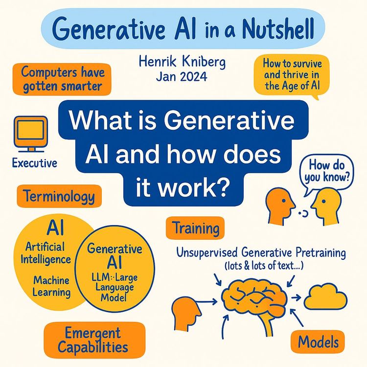
Video Course: What is Generative AI and how does it work?

Video Course: How to Use ChatGPT from Beginner to Professional

Video Course: How to Use Google Gemini for Google Workspace to Boost Productivity

Video Course: How to Use Claude 3.7 AI - Tips for Beginners!

Video Course: ChatGPT for Data Analytics: Full Course - from Beginners to Professional

Video Course: Generating Images and photos With ChatGPT?

Video Course: Generating Images & Photo's with MidJourney

Video Course: Generating Design's with Microsoft Designer and AI

Video Course: Generating Design's with Canva.com and AI
Join 20,000+ Professionals, Using AI to transform their Careers
Join professionals who didn’t just adapt, they thrived. You can too, with AI training designed for your job.