Become an AI Researcher: Math, PyTorch, LLMs & Transformers (Video Course)
Go from Python basics to reading papers and building GPT-style models. Learn the math that makes training work, code it in PyTorch, fix shape bugs, and ship ideas. If you want to contribute,not just watch,this path shows you how.
Related Certification: Certification in Building & Deploying LLMs and Transformers with PyTorch

Also includes Access to All:
What You Will Learn
- Apply calculus and linear algebra: derivatives, gradients, matrices, probability
- Use PyTorch tensors: reshape, slice, matmul, GPU ops, and autograd
- Implement neurons and multi-layer networks with forward/backward passes
- Build self-attention: Q/K/V, scaled dot-product, causal masking, multi-head attention
- Assemble and train a decoder-only GPT with positional embeddings and FFNs
- Prototype, debug, and evaluate research ideas using checkpoints and perplexity
Study Guide
Become an AI Researcher: LLM, Math, PyTorch, Neural Networks, Transformers
Let's be honest: if you want to do real AI research,not just use AI tools,you need to master the language under the hood. That language is math. Then you need a medium to express it,PyTorch. From there, you'll build up the mental models of neurons, layers, and loss functions, and graduate to the architecture that powers modern intelligence: the Transformer. This course is a complete, step-by-step guide that takes you from zero to reading papers, building models, and understanding exactly why they work,so you can contribute to the field instead of just watching it.
We'll start with foundations: functions, derivatives, vectors, gradients, matrices, and probability. Then we'll translate that into code with tensors, tensor operations, and GPU-backed matrix multiplications in PyTorch. You'll assemble single neurons into multi-layer networks, learn how backpropagation actually computes updates, and then go deep on attention, positional embeddings, and GPT-style decoder-only models. If you commit to the sequence, you'll leave with the cognitive tools to read research, implement ideas, debug models, and propose your own improvements.
How to Use This Course
Prerequisites are simple: basic Python,variables, lists/arrays, loops, and functions. If you can read and write simple Python, you can learn the rest here. Install NumPy, Matplotlib, and PyTorch. That's enough to build and visualize core ideas.
Learning objectives you'll hit by the end:
- Understand the math behind AI: functions, derivatives, vectors, gradients, matrices, probability.
- Define and manipulate tensors in PyTorch: reshaping, slicing, matrix multiplication, and broadcasting.
- Explain neurons, weights, biases, activation functions, and multi-layer forward passes.
- Describe and implement attention (Q, K, V), self-attention, multi-head attention, and masking.
- Outline and implement a GPT-style decoder-only transformer model,and know how to train it in practice.
Part 1 , Mathematics Is the Language of AI
AI is applied mathematics. Derivatives, gradients, and matrix multiplication aren't theory for theory's sake,they're the exact tools used to make models learn. If a paper confuses you, it's almost always because there's a gap in one of these topics. Close the gap, and the paper becomes readable.
Functions: Linear and Non-Linear
A function maps inputs to outputs. That's the essence of a neural network: a (very large) function that maps data to predictions.
Linear Functions (y = mx + b)
- m is the slope (how fast the output changes with x). b shifts the entire line up or down.
- In models, this is exactly what a neuron does before the activation: linear transformation plus bias.
Non-Linear Functions
- Quadratic (y = x²): accelerates as x moves away from zero.
- Cubic (y = x³): steeper growth for large |x| and preserves sign.
- Exponential (y = a^x): grows explosively; useful to understand why softmax can saturate.
Example 1:
A sensor's temperature reading x is converted to a system output y with y = 2x + 5. Doubling the slope makes the system twice as sensitive to changes in x.
Example 2:
A quadratic cost y = (x - 3)² penalizes values of x farther from 3. Moving from x = 2 to x = 1 increases cost from 1 to 4,non-linear growth in penalty.
Practical application: Most layers compute y = Wx + b. That's a matrix of linear functions. Without non-linear activations after it, stacking layers would just collapse to another linear function. Non-linearity is the difference between a toy and an intelligent system.
Derivatives: Rates of Change
A derivative tells you how fast a function changes at a point. In training, it tells you how changing a weight changes the error.
- Power rule: d/dx of xⁿ = n xⁿ⁻¹.
- Linear functions have constant derivatives (y = 2x => derivative 2).
- Non-linear functions have derivatives that depend on x (y = x² => derivative 2x).
Example 1:
For y = x³, dy/dx = 3x². At x = 2, the slope is 12. At x = 0.5, it's 0.75. Changes in x near 2 affect y far more than changes near 0.5.
Example 2:
Loss L(w) = (w - 4)². dL/dw = 2(w - 4). If w = 10, gradient is 12 (it's "pushing" you back toward 4). If w = 3, gradient is -2 (nudging you up).
Tip: Always ask "slope at this point." That instinct helps you predict how parameters will update after each step.
Vectors: Direction, Magnitude, and Similarity
Vectors store features, embeddings, and parameters. They have direction and length (magnitude). Operations include addition, scaling, and dot product.
- Addition: element-wise.
- Scalar multiplication: stretches or compresses magnitude and flips direction with negative scalars.
- Magnitude: ||v|| = sqrt(sum of squares).
- Normalization: v / ||v|| gives a unit vector (length 1). Crucial for stability and comparability.
- Dot product: measures alignment/similarity between two vectors. Positive means similar direction; zero means orthogonal; negative means opposing.
Example 1:
v = [3, 4]. Magnitude = sqrt(3² + 4²) = 5. Normalized v̂ = [0.6, 0.8]. This keeps direction but standardizes length, which is helpful when comparing vectors.
Example 2:
Similarity: [1, 0] . [cos θ, sin θ] = cos θ. The dot product directly encodes angular similarity. In attention, dot(Q, K) says "how aligned are these representations?"
Application in LLMs: Word embeddings are vectors. The dot product between embeddings often reflects semantic similarity. That's why cosine similarity is a common retrieval metric.
Gradients: Multi-Dimensional Derivatives
For a function of many variables, the gradient is the vector of all partial derivatives. It points in the direction of steepest increase.
- Gradient descent: Move parameters in the opposite direction of the gradient of the loss to reduce error.
- Intuition: Picture standing on a hill made of error. The gradient points uphill; you step downhill.
Example 1:
f(x, y) = x² + y². Gradient ∇f = [2x, 2y]. At (3, 4), ∇f = [6, 8], pointing straight away from the origin. Minimization pulls you back toward (0, 0).
Example 2:
Loss L(w1, w2) = (w1 - 1)² + 10(w2 - 2)². ∇L = [2(w1 - 1), 20(w2 - 2)]. The steeper curvature in w2 demands smaller steps to avoid overshooting. That leads to the idea of adaptive optimizers.
Best practice: Learning rate must be appropriate for the curvature of the loss landscape. Too large and you oscillate or blow up. Too small and you crawl.
Matrices: The Workhorse of Deep Learning
Matrices represent batches, layers, and transforms. Matrix multiplication is the core compute unit for GPUs.
- Multiplication rule: (A is m×n) times (B is n×p) yields (m×p). Inner dimensions must match.
- Each element (i, j) of AB is the dot product of row i of A with column j of B.
- Transpose: swap rows and columns (Aᵀ).
- Identity matrix I: AI = A. It's the "1" of matrix algebra.
Example 1:
Input X (batch 2, features 3):
[ [1, 2, 3], [4, 5, 6] ]
Weights W (3×2):
[ [1, 0], [0, 1], [1, 1] ]
Output XW (2×2):
Row 1 . W = [1*1+2*0+3*1, 1*0+2*1+3*1] = [4, 5]
Row 2 . W = [4*1+5*0+6*1, 4*0+5*1+6*1] = [10, 11]
Example 2:
Activation stacking: y = ReLU(XW + b). XW is one matmul. Broadcasting adds bias b. ReLU applies element-wise. This is the default rhythm of a forward pass.
Tip: Respect shapes. Most implementation errors are mismatched dimensions. Write them down. If you can't track shapes on paper, you'll fight silent bugs in code.
Probability: Reasoning Under Uncertainty
Models output probabilities over classes or tokens. You'll use expectations, conditional probabilities, and the Law of Large Numbers.
- Probability: from 0 to 1.
- Expected value: the long-run average of a random variable.
- Conditional probability P(A|B): probability of A given B.
- Law of Large Numbers: empirical averages converge to expected values as sample size grows.
Example 1:
Expected value of a fair die: (1+2+3+4+5+6)/6 = 3.5. Simulating thousands of rolls approaches 3.5.
Example 2:
P(Rain|Cloudy) vs P(Rain). If it's cloudy, rain is more likely. In modeling terms, conditional dependencies matter for sequences and classification.
Application: Softmax turns logits into a categorical probability distribution. Cross-entropy loss uses probability theory to measure how well predicted distributions match targets.
Part 2 , PyTorch Fundamentals
PyTorch is how we translate math into working systems. Its core structure is the tensor,like a NumPy array with superpowers: GPU acceleration and automatic differentiation.
Tensors: What They Are and Why They Matter
Tensors are n-dimensional arrays. Scalars (0D), vectors (1D), matrices (2D), and higher dimensions for batches, channels, heads, and sequence lengths.
Example 1:
Create common tensors:
torch.ones(3, 4) -> 3×4 ones
torch.zeros(2, 2) -> 2×2 zeros
torch.rand(2, 3) -> random 2×3
Example 2:
Convert from NumPy:
arr = numpy.array([[1, 2], [3, 4]])
t = torch.from_numpy(arr) # shares memory
Tip: Move tensors to GPU when available for speed:
device = torch.device("cuda" if torch.cuda.is_available() else "cpu")
t = t.to(device)
Tensor Shape Skills: Flatten, Reshape, View, Squeeze, Unsqueeze, Transpose, Permute
Shape manipulation is constant in model building. Get comfortable transforming tensors without copying data when possible.
- flatten(): collapse dimensions into 1D.
- reshape()/view(): change shape without changing data. view() shares memory if contiguous; reshape() may copy.
- squeeze()/unsqueeze(): remove/add size-1 dimensions.
- transpose(): swap two dims; permute(): reorder multiple dims in any arrangement.
Example 1:
x = torch.rand(2, 3, 4)
x_flat = x.flatten(start_dim=1) # shape (2, 12)
x_squeezed = torch.rand(1, 3, 1).squeeze() # shape (3)
Example 2:
x = torch.rand(32, 10, 64) # (batch, seq, hidden)
x_t = x.transpose(1, 2) # (batch, hidden, seq)
x_perm = x.permute(1, 0, 2) # (seq, batch, hidden) for recurrent/attention code
Best practice: After permute or transpose, call contiguous() before view if you need a memory-contiguous layout.
Indexing, Slicing, and Boolean Masking
Access sub-tensors cleanly to manipulate inputs, filter items, or select batches.
Example 1:
x = torch.arange(12).reshape(3, 4)
row0 = x[0, :] # first row
first_two_cols = x[:, :2]
Example 2:
mask = x % 2 == 0
evens = x[mask] # select even elements
Tip: Use advanced indexing to gather specific indices across batches for attention or vocabulary lookups.
Concatenation, Stacking, and Matrix Multiplication
- torch.cat([t1, t2], dim): join along an existing dimension.
- torch.stack([t1, t2], dim): create a new dimension and stack.
- torch.matmul(a, b) or a @ b: matrix multiplication with broadcasting rules.
Example 1:
a = torch.ones(2, 3); b = torch.zeros(2, 3)
cat0 = torch.cat([a, b], dim=0) # shape (4, 3)
cat1 = torch.cat([a, b], dim=1) # shape (2, 6)
Example 2:
X = torch.rand(32, 128) # batch 32, features 128
W = torch.rand(128, 64)
Y = X @ W # (32, 64) , one layer's linear transform
Best practice: Keep a mental model of shapes at each step. Print shapes during debugging; it's faster than guessing.
Autograd: Differentiation Without Pain
PyTorch tracks operations on tensors with requires_grad=True, building a computation graph. Backward() computes gradients for all parameters.
Example 1:
w = torch.randn(3, 3, requires_grad=True)
x = torch.randn(3, 1)
y = w @ x
loss = y.pow(2).sum()
loss.backward() # now w.grad holds dloss/dw
Example 2:
Turn off grad during evaluation or with fixed embeddings:
with torch.no_grad():
y_pred = model(x)
Tip: Zero out gradients each step (optimizer.zero_grad()) to avoid accumulation.
Part 3 , Neural Networks: From Neuron to Deep Models
At its core, a neural network is a chain of linear transforms plus non-linear activations. The magic is in the scale, the architecture, and the optimization details.
The Single Neuron
A neuron computes a weighted sum of its inputs and adds a bias, then pushes it through a non-linear activation.
- Weighted sum: z = w . x + b.
- Output: a = activation(z).
- Weights and biases are learned by minimizing loss.
Example 1:
x = [0.5, 1.0, -0.5], w = [2.0, -1.0, 0.5], b = 0.1
z = (0.5*2.0) + (1.0*(-1.0)) + (-0.5*0.5) + 0.1 = -0.15
Example 2:
If activation is ReLU, a = max(0, -0.15) = 0. If activation is sigmoid, a ≈ 0.4625. Different activations produce different behaviors.
Practical note: A neuron without activation is just a linear equation. Stack a thousand of them without non-linearity and it's still a linear map.
Activation Functions
These inject non-linearity. They enable neural networks to model curved decision boundaries and complex patterns.
- Sigmoid: squashes to (0, 1). Useful for probabilities; saturates at extremes.
- ReLU: f(x) = max(0, x). Efficient and widely used.
- Leaky ReLU: small slope for x < 0 to prevent dead neurons.
Example 1:
ReLU on [-2, -0.1, 0, 0.3, 2] => [0, 0, 0, 0.3, 2]. Fast, sparse activations help training.
Example 2:
Sigmoid on large positive inputs approaches 1, and large negative inputs approach 0. That's why gradients vanish for extreme logits without care.
Tip: For deep nets, ReLU-like or GELU activations are common. For output layers, match activation to task (sigmoid for binary, softmax for multi-class, linear for regression).
Multi-Layer Networks and Forward Pass
Stack layers to build capacity. Each layer: y = activation(XW + b). The forward pass pushes input through all layers to produce outputs.
Example 1:
Two-layer MLP: hidden = ReLU(X @ W1 + b1); out = hidden @ W2 + b2. This can approximate complex functions with enough hidden units.
Example 2:
Batch processing: X is (batch, features). W1 is (features, hidden). W2 is (hidden, output). Outputs are (batch, output). Shapes tell the story.
Best practice: Use normalization (BatchNorm or LayerNorm) to stabilize training in deeper stacks.
Loss Functions and Optimization
Loss quantifies error. Optimization adjusts parameters to minimize it.
- Common losses: MSE for regression, Cross-Entropy for classification.
- Optimizers: SGD, Momentum, Adam. They differ in how they use gradients to step through the loss landscape.
Example 1:
Binary cross-entropy: L = -[y log(p) + (1 - y) log(1 - p)]. If the model assigns high probability to the correct label, loss is small.
Example 2:
For multi-class with softmax, cross-entropy penalizes confident wrong predictions heavily, encouraging correct class probability to grow.
Tip: Start with Adam and a moderate learning rate, then tune. For very large models or datasets, learning rate scheduling helps (warmup, cosine decay).
Backpropagation and the Chain Rule
Backpropagation computes gradients layer-by-layer from the output back to the input using the chain rule. It's how every parameter learns how to change.
Example 1:
If out = f(g(h(x))), then dL/dx = (dL/df).(df/dg).(dg/dh).(dh/dx). This is the chain rule in action, exactly what autograd does for you.
Example 2:
In a two-layer network, gradients flow through W2 back into hidden activations and then through W1 to inputs. This helps you reason about vanishing or exploding gradients.
Best practice: Initialize weights carefully (e.g., Kaiming for ReLU). Use residual connections and normalization in deep networks to maintain healthy gradient flow.
A Minimal Training Loop in PyTorch
You'll repeat this pattern in every model you train.
Example 1:
for batch in loader:
optimizer.zero_grad()
y_pred = model(x)
loss = criterion(y_pred, y_true)
loss.backward()
optimizer.step()
Example 2:
Evaluation loop with no grad and metrics tracking:
with torch.no_grad():
y_pred = model(x_val)
val_loss = criterion(y_pred, y_val)
Tip: Clip gradients (torch.nn.utils.clip_grad_norm_) if you see explosions. Log everything: loss curves, learning rate, and validation metrics.
Common Pitfalls and Stability Tips
- Vanishing gradients: use ReLU-like activations, residual connections, and proper initialization.
- Exploding gradients: gradient clipping, smaller learning rate, normalization.
- Overfitting: regularization, dropout, early stopping, more data augmentation.
- Shape errors: print shapes liberally; write small tests for layers.
Part 4 , Transformers and Large Language Models (LLMs)
Transformers replaced recurrence by letting models attend to any token in the sequence. Context is no longer limited by step-by-step memory,it's computed through attention.
Why Attention Exists
Language is context. A word can mean different things depending on other words around it. Attention lets the model decide which tokens matter most for each prediction.
Example 1:
"The bank near the river…" vs "The bank approved the loan…" The word "bank" is clarified by different context tokens. Attention learns those relationships.
Example 2:
Long-range dependencies: "The book that you gave me yesterday was incredible." The subject "book" and "was" are separated by several tokens. Attention bridges that gap.
Q, K, V: The Mechanics of Self-Attention
Each input token embedding is linearly projected to three vectors: Query (Q), Key (K), and Value (V).
- Query: what this position is looking for.
- Key: what information this position offers.
- Value: the content to share.
Scaled dot-product attention pipeline:
1) Compute scores = QKᵀ / sqrt(dk).
2) Apply mask if needed (for causal models).
3) Softmax over scores to get attention weights.
4) Weighted sum: weights @ V gives contextualized representations.
Example 1:
Toy scenario with 3 tokens, dk = 2. If Q for token 2 has a high dot product with K of token 1 and low with token 3, then token 2 will attend mostly to token 1. After softmax, weights might be [0.7, 0.25, 0.05] over [1,2,3].
Example 2:
Similarity: dot(Q, K) works like the vector dot product you learned earlier,this is literally how affinity is measured before softmax.
Best practice: Always scale by 1/sqrt(dk). It prevents extremely large dot products from collapsing the softmax distribution into near one-hot vectors too early.
Scaled Dot-Product, Softmax, and Causal Masking
- Scaling: normalize scores by sqrt(dk) for stability.
- Softmax: converts raw scores to a probability distribution over tokens (weights that sum to 1).
- Causal mask: forbid attending to future tokens in next-token prediction to avoid "cheating."
Example 1:
Mask matrix is upper triangular with -inf above the diagonal. After adding to scores and applying softmax, weights for future positions become 0.
Example 2:
In training, the model sees input "The cat sat on the" and predicts next token. Causal masking ensures "mat" remains hidden when predicting "the."
Multi-Head Attention
Instead of one attention operation, run multiple heads in parallel with different learned Q/K/V projections. Each head captures different relationships,syntax, coreference, long-term dependencies, etc.
Example 1:
Head 1 focuses on subject-verb agreement. Head 2 focuses on noun-adjective bindings. Combined, the model captures richer structure.
Example 2:
In code: split hidden dimension into H heads, apply attention in each head, then concatenate heads and apply a final linear projection to re-mix information.
Tip: Head dimension must divide the hidden size. Typical choice is d_model = H * d_head.
Positional Embeddings: Order Matters
Self-attention alone is permutation-invariant. We inject position information so the model understands order.
- Absolute positional embeddings: add a learned vector for each position index.
- Rotary Positional Embeddings (RoPE): rotate pairs of embedding dimensions by a position-dependent angle, encoding relative positions elegantly.
Example 1:
Absolute: position 0 gets pos_vec0 added to token embedding, position 1 gets pos_vec1, and so on. The model learns positional patterns during training.
Example 2:
RoPE: if you think of embedding dimensions paired like complex numbers, each position rotates the vector by a fixed angle frequency. This lets attention naturally model distances and extrapolate better to longer sequences.
Tip: For longer context windows, RoPE often performs well compared to classic sinusoidal embeddings because it maintains relative position information within dot products.
Feed-Forward Networks in Each Block
After attention, each token passes through the same two-layer MLP with a non-linearity (often GELU). This is applied independently to each token's vector.
Example 1:
FFN: z = activation(xW1 + b1); out = zW2 + b2. Typically W1 expands dimensionality (e.g., 4× hidden), then projects back down.
Example 2:
Interpretation: Attention gathers information; FFN transforms and stores it. Many factual associations end up encoded in these feed-forward layers.
Tip: The expansion ratio (e.g., 4x) is a strong lever for capacity and compute. Bigger FFNs can store more "knowledge."
Residual Connections and Layer Normalization
Each sub-layer (attention or FFN) has a residual connection (Add) followed by LayerNorm (Norm). This stabilizes training and keeps gradients healthy through depth.
Example 1:
y = LayerNorm(x + Attention(x)). Skip connections allow the model to learn perturbations of the identity map rather than full transformations from scratch.
Example 2:
y = LayerNorm(x + FFN(x)). The identity path helps gradients flow. Without it, deep transformers are much harder to train.
Tip: Pre-norm transformers (LayerNorm before attention/FFN) are common because they improve stability and training speed.
Decoder-Only GPT Stack
A GPT-style model stacks N transformer blocks using causal self-attention only. Final token embeddings are projected to vocabulary logits with a linear layer.
- Input tokens -> token embeddings (+ positional or rotary) -> stacked blocks (attention + FFN with residuals and norms) -> linear projection to vocab -> softmax for probabilities.
Example 1:
Inference loop: feed in "The cat sat," get distribution for next token; sample "on"; append and repeat. The model writes one token at a time.
Example 2:
Training: feed sequence "[The, cat, sat, on, the]" and teach the model to predict "[cat, sat, on, the, mat]." Causal mask ensures each token only attends to earlier ones.
Tip: Tie input and output embeddings to save parameters and often improve performance slightly.
Outline: Building a Minimal GPT in PyTorch
Here's a high-level blueprint you can implement, block by block.
Example 1:
Tokenization and embeddings:
- Map text to integer token IDs (vocab).
- token_emb = Embedding(vocab_size, d_model)
- pos or RoPE added/applied.
Example 2:
Transformer block:
- LayerNorm -> Multi-Head Attention with causal mask -> residual add.
- LayerNorm -> FFN (d_model -> 4*d_model -> d_model) -> residual add.
Example 3:
Forward pass:
- x = token_emb(tokens)
- x = apply_positional_encoding(x)
- for each block: x = block(x)
- logits = x @ W_vocab # project to vocabulary size
- loss = CrossEntropyLoss(logits, targets)
Example 4:
Training steps:
- Create batches of contiguous token windows (context_length).
- optimizer.zero_grad(); loss.backward(); optimizer.step().
- Use learning rate warmup and decay; clip gradients if needed.
Best practices:
- Check all tensor shapes at each step (batch, seq, d_model).
- Ensure causal masks are correct,most silent failures come from incorrect masking.
- Mixed precision (autocast, GradScaler) can speed training on GPU significantly.
Training Tips: Data, Batching, and Evaluation
- Data pipeline: clean text, tokenize, build fixed-length sequences (overlapping windows to maximize usage).
- Batch size: tune based on memory. Accumulate gradients if needed.
- Learning rate: start small; use warmup steps then decay. Cosine annealing works well.
- Evaluation: use perplexity for language modeling; track validation loss frequently.
Example 1:
Batching contiguous segments: take a long tokenized corpus, create windows of length T as inputs and the next T tokens as targets. Slide by T or with overlap.
Example 2:
Checkpointing: save model state_dict, optimizer state, and step counter. Resume training cleanly and evaluate regularly to avoid regressions.
Key Insights You Must Internalize
Mathematics is the language.
Derivatives, gradients, and linear algebra aren't optional,they are the mechanisms of learning and computation.
Matrix multiplication is core.
Neural networks are sequences of matrix multiplications plus element-wise functions, massively parallelized on GPUs.
Gradients drive learning.
They point uphill; we move parameters downhill to minimize error via gradient descent.
Activation functions enable complexity.
They let models go beyond linear mappings and fit real-world data structures.
Attention is about context.
The dot product between query and key measures affinity. Softmax turns those scores into weights that decide what to focus on.
The roadmap is sequential.
Math → PyTorch → neural networks → transformers. Master each layer; don't skip ahead.
Implications and Applications
For education and self-study:
Use this sequence as your syllabus. Don't just memorize formulas; derive them for small examples. Implement each concept in PyTorch. Code a single neuron, then a layer, then a small MLP, then an attention block. The mental muscle you build will make papers feel simpler.
For research and development:
You'll need intuition for gradients to troubleshoot vanishing or exploding issues, comfort with tensor shapes to diagnose bugs, and confidence to read and implement novel ideas. When you see a paper propose a new attention variant or normalization tweak, you should be able to prototype it and evaluate the result.
For policy and strategy:
Leaders can use this framework to understand skill sets on an AI team, separate hype from substance, and plan infrastructure investments around data pipelines, GPU allocation, and evaluation protocols.
Recommendations for Aspiring AI Researchers
1) Master the mathematical foundations.
Practice derivatives, gradients, and matrix multiplications by hand. Do small numeric examples. Confidence here pays off everywhere else.
2) Engage in hands-on practice.
Implement from scratch: a neuron, a linear layer, a mini-MLP, a single-head attention block, then multi-head attention and a transformer block.
3) Follow the structured path.
Resist the urge to jump directly to giant models. The basics compound. You'll go faster by going in order.
4) Connect theory to practice.
When you learn a concept, find it in a paper. Read sections slowly, rewrite equations in your own symbols, and code a minimal version to test your understanding.
Deep Dive: Every Core Concept with Extra Examples and Applications
To make sure everything is locked in, here are additional concrete examples for the most critical ideas.
More on Functions
Example 1:
Exponential growth: y = 2^x. From x = 3 to x = 4, y jumps from 8 to 16. From 10 to 11, it jumps from 1024 to 2048. That's why softmax can quickly saturate if logits are scaled too high.
Example 2:
Piecewise linearity: ReLU networks are piecewise linear functions. With enough pieces (neurons), they approximate highly complex curves.
Application: Activations are just non-linear functions. Your choice controls how representational capacity flows through the network.
More on Derivatives
Example 1:
Derivative of e^x is e^x. Meaning: the rate of change equals the value itself. In softmax and cross-entropy calculations, this derivative shows up repeatedly.
Example 2:
Chain rule in practice: If y = ReLU(Wx + b), then dy/dW depends on x, and dy/dx depends on W and the activation's derivative. That exact structure is what autograd computes.
More on Vectors and Dot Products
Example 1:
Orthogonality: [1, 0, 0] . [0, 1, 0] = 0. Completely unrelated directions. This is how you can think about keys and queries that shouldn't attend to each other.
Example 2:
Cosine similarity: cos_sim(u, v) = (u.v) / (||u|| ||v||). Normalize first, then dot. Clean metric for comparing embeddings from different sources.
More on Gradients and Descent
Example 1:
Stochastic gradient descent (SGD): updates based on small random batches lead to noisy but efficient movement toward minima. The noise can help escape shallow local minima.
Example 2:
Adam optimizer uses running averages of gradients and squared gradients to adapt learning rates per parameter. Great for sparse or noisy problems.
More on Matrices
Example 1:
Broadcasting bias: XW + b uses broadcasting to add b to each row of XW. Saves memory and code complexity.
Example 2:
Batching through matrix math: stacking multiple inputs into a batch lets GPUs parallelize matmuls massively. That's where real speed comes from.
More on Probability
Example 1:
Softmax: p_i = exp(z_i)/sum_j exp(z_j). If z increases by +c for all i, probabilities don't change,that's why you can subtract max(z) before softmax for numerical stability.
Example 2:
Confidence calibration: A model that predicts 0.9 probability and is correct 90% of the time is well calibrated. Temperature scaling adjusts logits to improve calibration.
Transformers: Extra Attention Examples
Example 1:
Scaled dot-product: if dk = 64 and unscaled dot products are on average around 8, dividing by sqrt(64) = 8 brings scores to ~1, preventing softmax from collapsing.
Example 2:
Multi-head composition: one head focuses on nearby tokens, another on far-away tokens. The concatenated output mixes short- and long-range context efficiently.
Outline to Train a GPT-Style Model (Step-by-Step)
1) Data: collect and clean text. Tokenize into integer IDs. Build a vocabulary.
2) Windows: create fixed-length sequences of length T for inputs; targets are inputs shifted by one.
3) Model: token embeddings + (RoPE or learned positions) + N decoder blocks (each: LayerNorm, causal multi-head attention, residual; LayerNorm, FFN, residual).
4) Objective: cross-entropy loss over next-token predictions.
5) Optimization: AdamW with weight decay; learning rate warmup then decay; gradient clipping.
6) Evaluation: measure validation loss and perplexity; sample outputs to qualitatively inspect behavior.
7) Iteration: tune context length, number of layers/heads, hidden size, and FFN expansion for performance and compute budget.
Example 1:
If T = 128, batch_size = 64, your input tensor is (64, 128). Embedding produces (64, 128, d_model). Every block preserves (64, 128, d_model). Final linear maps to (64, 128, vocab_size).
Example 2:
To generate: start with a prompt, repeatedly sample from the last position's distribution, append the sampled token, and continue until you hit max length or an end token.
Authoritative Statements (Internalize These)
Statement:
Gradients are how neural networks learn. They show the direction of steepest ascent for the loss, and we step in the opposite direction to minimize error.
Statement:
Neural networks are sequences of matrix multiplications executed quickly and efficiently on GPUs. That's the backbone of modern deep learning.
Statement:
The derivative of a function shows its rate of change. In a neural network, it tells you exactly how a small change in a weight will influence the loss.
Statement:
The dot product measures vector similarity. High dot products between queries and keys signal high affinity and lead to strong attention weights.
Best Practices and Research Habits
- Always connect a new idea to a simple numeric example. If you can't compute a tiny case by hand, you don't fully own it yet.
- Keep a shape diary: write dimension flows for each layer. This isolates bugs and makes you fast.
- Inspect activations and gradients. Plot distributions. Watch for dead ReLUs or exploding statistics.
- Read landmark papers slowly. Re-derive a few equations, implement a minimal version, and test with toy data.
- Build intuition with ablations: turn features off and on to see what matters (heads, FFN expansion, normalization placement).
Final Checklist: Did We Cover Every Core Point?
- Functions: linear and non-linear with multiple examples and applications.
- Derivatives: concept, power rule, role in optimization.
- Vectors: addition, scaling, magnitude, normalization, dot product, and interpretation.
- Gradients: multi-dimensional derivative, steepest ascent, gradient descent.
- Matrices: multiplication, transpose, identity, and their role in layers and batches.
- Probability: expected value, conditional probability, Law of Large Numbers, and softmax implications.
- PyTorch tensors: creation, flatten, reshape/view differences, squeeze/unsqueeze, transpose/permute.
- Indexing, slicing, boolean masks; concatenation, stacking, and matmul.
- Single neuron: weights, bias, activation; activation functions (sigmoid, ReLU, Leaky ReLU).
- Multi-layer networks: forward pass and matrix view.
- Backpropagation: chain rule and optimizer flow.
- Transformers: attention mechanism, Q/K/V, scaling, softmax, causal masking.
- Multi-head attention, positional embeddings (including RoPE), FFN, residuals, and layer normalization.
- GPT-style decoder-only architecture: stacked blocks, final linear projection to vocabulary.
- Practical implementation outline and training tips.
- Key insights, implications, and recommendations for your study path.
Conclusion: Build, Test, Iterate
You now have the roadmap: math first, tensors next, neurons into networks, and attention through transformers. The whole field opens up once you can translate equations into code and back again. Practice isn't optional,implement a neuron, a layer, a tiny MLP, then a minimal attention block, then stack a few blocks with causal masking. Train on small text, measure perplexity, and iterate.
Your edge won't come from memorizing buzzwords. It comes from internalizing derivatives, gradients, and matrix multiplications; from manipulating tensors with ease; from understanding why attention weights look the way they do; from diagnosing training behavior and fixing it with the right tool. Keep your curiosity high, your experiments small and frequent, and your shape notes close. That's how you go from using AI to contributing to it,and that's how you become an AI researcher who builds things that matter.
Frequently Asked Questions
This FAQ helps you turn curiosity into working models. It starts with the essentials (math, tensors, and neurons), moves into Transformers and LLMs, and finishes with training, evaluation, deployment, and business impact. The focus is practical: clear definitions, common pitfalls, and examples you can map to real products and research.
Getting Started
What prerequisites do I need to succeed?
Core skills:
Comfortable Python, basic NumPy, and high-level math intuition (functions, derivatives, vectors, matrices, and probability). You don't need to be a mathematician; you need to read formulas, translate them to code, and reason about outputs.
Tools:
Install PyTorch, NumPy, and Matplotlib. Use a GPU if possible (local or cloud). A code editor with Python linting and a notebook environment (Jupyter or VS Code) speeds iteration.
Mindset:
Work in small experiments. Read papers, then re-implement minimal versions. Debug shapes first, then logic. Learn to profile performance and memory early.
Business angle:
Map concepts to use cases: classification for churn, sequence models for support routing, and Transformers for summarization. The goal is not theory for theory's sake,it's reliable decision-making and product features backed by measurable results.
Foundational Mathematics for AI
What are the key mathematical concepts for AI research?
The essentials:
Functions, derivatives, vectors, gradients, matrices, and probability are the backbone. Functions map inputs to outputs. Derivatives and gradients show how to change weights to reduce loss. Vectors and matrices represent data and parameters efficiently. Probability helps interpret uncertainty and outputs.
Why it matters:
Every forward pass is matrix multiplication; every update is gradient-based. If you can parse shapes, compute dot products, and reason about rate of change, you can debug almost anything.
Example:
In a marketing uplift model, gradients adjust weights to minimize cross-entropy loss. Matrix ops let you score thousands of customers at once. Probability turns logits into actionable likelihoods (e.g., probability a user churns).
What is a derivative and how is it used in neural networks?
Concept:
A derivative is the slope of a function at a point. For y=2x, the slope is constant (2). For y=x², the slope is 2x and changes with x.
In practice:
Neural networks use derivatives during backpropagation to learn. The derivative of the loss with respect to each weight tells you how much and in which direction to adjust that weight to reduce error. Optimizers (like AdamW) scale these updates across steps.
Example:
If your model predicts product demand too high, the derivative of the loss with respect to weights nudges them down, gradually aligning predictions with reality. This is gradient descent in action,small, consistent steps guided by derivatives.
What is a vector and why is it fundamental to machine learning?
Definition:
A vector is an ordered list of numbers with magnitude and direction. It's the universal container for data: text embeddings, image pixels, user features, and parameters.
Why it matters:
Vectors enable fast, parallel computation and geometric reasoning (similarity, distance, projection). Operations like dot product and normalization are essential for attention, recommendations, and feature scaling.
Examples:
* Word embeddings: a 768-dimensional vector capturing semantics.
* Customer profile: spend, frequency, recency,packed into a vector for scoring.
* Attention: query and key vectors' dot product measures relevance, guiding which tokens to focus on.
How do you calculate the length (magnitude) of a vector?
Formula:
Magnitude = sqrt(sum of squared elements). For [3,4], that's sqrt(3²+4²)=5. This generalizes to any dimension.
Why it matters:
Magnitude informs normalization, distance metrics, and stability. Without it, comparisons across samples or features can be misleading.
Example:
When ranking similar documents by cosine similarity, you normalize vectors to unit length so ranking depends on direction (semantics), not raw scale. This keeps nearest-neighbor search consistent across documents of different lengths.
What is vector normalization and why is it important?
Definition:
Normalization scales a vector to length 1 by dividing by its magnitude. Direction stays the same; size becomes uniform.
Why it matters:
It reduces exploding/vanishing effects, stabilizes training, and makes comparisons fair. Many similarity measures (cosine) assume unit vectors.
Real-world use:
* Search: normalize embeddings before approximate nearest-neighbor search for better relevance.
* Training: normalized inputs and gradients help models converge faster and more reliably.
* Recommenders: compare user and item vectors without bias toward high-variance users.
What does the dot product of two vectors represent?
Meaning:
The dot product measures alignment. Positive means similar direction, zero means orthogonal, negative means opposing. Numerically, it's the sum of elementwise products.
Where it shows up:
Attention scores (Q.K), linear layers, similarity searches, and projections. It's the core of how Transformers decide which tokens influence each other.
Example:
In a support bot, the user's question embedding dotted with knowledge-base embeddings ranks the most relevant article. A higher dot product signals stronger relevance and higher display priority.
What is a gradient and what is its role in training neural networks?
Definition:
A gradient is the vector of partial derivatives of the loss with respect to parameters. It points in the direction of steepest increase; we step in the opposite direction to reduce loss.
Usage:
Compute gradients via backprop, then apply an optimizer (e.g., AdamW) to update weights. Repeat across batches and epochs until convergence or early stopping triggers.
Example:
Optimizing a sales-forecast model: after each batch, gradients indicate how each weight affected error. Updates move the model toward lower forecast error, improving inventory planning.
What are the rules for matrix multiplication and why is it a core operation in AI?
Rules:
Shapes must align: (m×n).(n×p) → (m×p). Each output element is a dot product of a row in the first matrix and a column in the second. It's not commutative (A.B ≠ B.A).
Why it matters:
Every layer's forward pass is matrix multiplication: inputs × weights (+ bias). GPUs accelerate these ops at massive scale.
Example:
Batching 1,024 sentences through a Transformer multiplies large activation matrices by weight matrices efficiently, enabling fast training and inference.
How is probability used in AI and LLMs?
Core idea:
Models output distributions over classes or tokens. Probability quantifies uncertainty and guides decisions (thresholds, risk trade-offs).
Applications:
* Classification: convert logits to probabilities, then pick a class or set a threshold (e.g., fraud alert if P>0.8).
* Language modeling: next-token probabilities drive text generation and evaluation (perplexity).
* Calibration: align predicted probabilities with real outcomes for reliable decisions (e.g., medical triage).
Business fit:
Probability lets you price risk, set SLA fallbacks, and tune systems for precision vs. recall depending on cost of errors.
Certification
About the Certification
Get certified in AI Research: Math, PyTorch, LLMs & Transformers , prove you can read papers, build and train GPT-style models in PyTorch, fix shape bugs, evaluate results, and ship production-ready prototypes.
Official Certification
Upon successful completion of the "Certification in Building & Deploying LLMs and Transformers with PyTorch", you will receive a verifiable digital certificate. This certificate demonstrates your expertise in the subject matter covered in this course.
Benefits of Certification
- Enhance your professional credibility and stand out in the job market.
- Validate your skills and knowledge in cutting-edge AI technologies.
- Unlock new career opportunities in the rapidly growing AI field.
- Share your achievement on your resume, LinkedIn, and other professional platforms.
How to complete your certification successfully?
To earn your certification, you’ll need to complete all video lessons, study the guide carefully, and review the FAQ. After that, you’ll be prepared to pass the certification requirements.
Other AI Video Courses
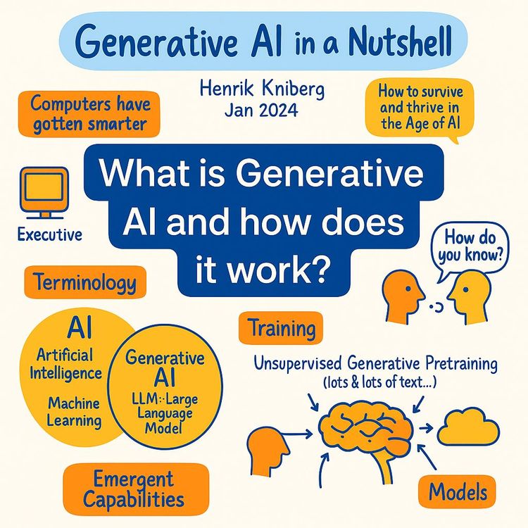
Video Course: What is Generative AI and how does it work?

Video Course: How to Use ChatGPT from Beginner to Professional

Video Course: How to Use Google Gemini for Google Workspace to Boost Productivity

Video Course: How to Use Claude 3.7 AI - Tips for Beginners!

Video Course: ChatGPT for Data Analytics: Full Course - from Beginners to Professional

Video Course: Generating Images and photos With ChatGPT?

Video Course: Generating Images & Photo's with MidJourney

Video Course: Generating Design's with Microsoft Designer and AI

Video Course: Generating Design's with Canva.com and AI
Join 20,000+ Professionals, Using AI to transform their Careers
Join professionals who didn’t just adapt, they thrived. You can too, with AI training designed for your job.